Intelligent Game Playing
770 likes | 792 Views
Dive into the evolution of game-playing machines, from "The Turk" in 1770 to IBM's Deep Blue defeating Garry Kasparov in 1997. Explore the Mini-Max algorithm and its application in games like chess, poker, and Go. Learn about Mini-Max for Nim games and its challenges, as well as the properties and limitations of the algorithm.

Intelligent Game Playing
E N D
Presentation Transcript
Intelligent Game Playing Instructor: B. John Oommen Chancellor’s Professor Life Fellow: IEEE; Fellow: IAPR School of Computer Science, Carleton University, Canada The primary source of these notes are the slides of Professor HweeTou Ng from Singapore. The Multi-Player Game section was due to Mr. Spencer Polk. I sincerely thank them for this.
Question: Can machines outplay humans? Captured imaginations for centuries Appearance in myth and legend Popular topic in fiction Thanks to AI and search techniques, the dream has come true! Games - Introduction
History • “The Turk”: In 1770 • A chess playing machine • Toured Europe • Facing well-known opponents • e.g. Napoleon, Ben Franklin • Of course: Revealed - fraud The Turk (1770)
History • “The Turk” shows how fascinating this idea is • 1914: King vs Rook strategies by automaton • True AI game playing – Claude Shannon: 1950 • Based on earlier work by Nash and Neumann • Shannon's algorithm still used • Mini-Max Search (we will return to it shortly)
History • Shannon's 1950 paper focused on Chess • Chess remains very important to game playing research • At the time, seen as purely theoretical exercise • 1970s: First commercial Chess programs • 1980s: Chess programs playing at Expert level • Still some time until Grandmaster level...
History • 1997: IBM's Deep Blue • Defeats Garry Kasparov • First defeat of Grandmaster • Field: Branched out since • Poker, Go: Now important games • IBM Watson on Jeopardy Kasparov vs Deep Blue
Games vs. Search Problems • “Unpredictable” opponent • Specifying a move for every possible opponent reply • Time limits • Unlikely to find goal, must approximate
Mini-Max Search • Search to find the correct move in a two player game • The optimal solution: • Exponential algorithm • Generate all possible paths • Only play those that lead to a winning final position • Realistic alternative to the Optimal • Use finite depth look-ahead with a heuristic function • Evaluate how good a given game state is
Mini-Max • Extend Tree down to a given search depth • Top of tree is the Computer’s move • Wants move to ultimately be one step closer to a winning position • Wants move that maximizes own chance of winning • Next move is Opponent’s • Opponent assumed to perform a move that his best • Wants move that minimizes Computer’s chance of winning
Mini-Max • Perfect play for deterministic games • Idea: Choose move to position with highest Mini-Max value = Best achievable payoff against best play • Example: 2-ply game:
Mini-Max for Nim • Nim Game • Two players start with a pile of tokens • Legal move: Split (any) existing pile into two non-empty differently sized piles • Game ends when no pile can be unevenly split • Player who cannot make his move loses the game • Search strategy • Existing heuristic search methods do not work
Mini-Max for Nim • Label nodes as MIN or MAX, alternating for each level • Define utility function (payoff function). • Do full search on tree • Expand all nodes until game is over for each branch • Label leaves according to outcome • Propagate result up the tree with: • M(n) = max( child nodes ) for a MAX node • m(n) = min( child nodes ) for a MIN node • Best next move for MAX is the one leading to the child with the highest value (and vice versa for MIN)
Mini-Max Algorithm function MINIMAX-DECISION(game) returnsan operator for each opin OPERATORS[game] do VALUE[op] := MIN-VALUE(APPLY(op, game), game) end return the op with the highest VALUE[op] function MAX-VALUE(state, game) returnsa utility value if CUTOFF-TEST(state,) then return EVAL(state) value := - ∞ for each sin SUCCESSORS(state) do value := MAX(value, MIN-VALUE(s, game)) end return value function MIN-VALUE(state, game) returnsa utility value if CUTOFF-TEST(state,) then return EVAL(state) value := ∞ for each sin SUCCESSORS(state) do value := MIN(value, MAX-VALUE(s, game)) end return value
Problems with Mini-Max • Horizon effect: Can’t see beyond depth • Due to exponential increase in tree size, only very limited depth feasible • Solution: Quiescence search. Start at the leaf nodes of the main search, and try to solve this problem. • In Chess, quiescence searches usually include all capture moves, so that tactical exchanges don't mess up the evaluation. In principle, quiescence searches should include any move which may destabilize the evaluation function--if there is such a move, the position is not quiescent. • May want to use look up tables • For end games • Opening moves (called Book Moves)
Properties of Mini-Max • Complete? • Yes (if tree is finite) • Optimal? • Yes (against an optimal opponent) • Time complexity? • O(bm) • Space complexity? • O(bm) (depth-first exploration) • Chess: b ≈ 35, m ≈100 for “reasonable” games • Exact solution completely infeasible
Branch and Bound: The α-β Algorithm • Branch and Bound: If current path (branch) is already worse then some other known path: • Stop expanding it (bound). • Alpha-Beta is a branch and bound technique for Mini-Max search • If you know that the level above won’t choose your branch because you have already found a value along one of your sub-branches that is too good, stop looking at other sub-branches that haven’t been looked at yet
The α-β Algorithm • Instead of maintaining a single mini-max value , the α-β pruning algorithm, maintains two: α, β • Together provide a bound on the possible values of the mini-max tree at any given point. • At any given point, α:minimum the player can expect to receive • At any given point, β:maximum value the player can expect
The α-β Algorithm • If it is ever the case that this bound is reversed or has range of 0 (β <= α), then better options exist for the player at other pre-explored nodes • As αis the minimum value we know we can get • Thus this node cannot be the mini-max value of the tree. • There is no point in exploring any more of this node's children • Potentially saving considerable computation time in a game with a large branching factor/depth
Properties of α-β • Pruning does not affect final result • Good move ordering improves pruning effectiveness • With “perfect ordering” time complexity = O(bm/2) • Doubles depth of search • α-β is a simple example of the value of reasoning about which computations are really relevant
Why it is called α-β • α: Value of the best choice found so far at any choice point along the path for max • If v is worse than α • max will avoid it • prune that branch • Define β similarly for min
The α-β Algorithm = best score for MAX so far = best score for MIN so far game = game description state = current state in game • From Russell and Norvig function MAX-VALUE(state, game, , ) returnsa utility value if CUTOFF-TEST(state,) then return EVAL(state) for each sin SUCCESSORS(state) do := MAX(, MIN-VALUE(s, game, ,)) if≥then return end return function MIN-VALUE(state, game, , ) returnsa utility value if CUTOFF-TEST(state,) then return EVAL(state) for each sin SUCCESSORS(state) do := MIN(, MAX-VALUE(s, game, ,)) if≤then return end return
Improving Game Playing • Increase Depth of Search • Have better heuristic for game state evaluation Changing Levels of Difficulty • Increase Depth of Search
Resource Limits • Suppose we have 100 secs, explore 104 nodes/sec • 106nodes per move • Standard approach: • Cutoff test: Depth limit (perhaps add quiescence search) • Evaluation function: • Estimated desirability of position
Evaluation Functions • Chess, typically linear weighted sum of features Eval(s) = w1 f1(s) + w2 f2(s) + … + wn fn(s) • Example: w1 = 9 with f1(s) = (number of white queens) – (number of black queens) etc.
Cutting-Off Search MinimaxCutoff is identical to MinimaxValue except • Terminal? is replaced by Cutoff? • Utility is replaced by Eval Does it work in practice? bm = 106, b=35 m=4 4-ply lookahead is a hopeless chess player! • 4-ply ≈ human novice • 8-ply ≈ typical PC, human master • 12-ply ≈ Deep Blue, Kasparov
Quiescence search • Quiescence search: Study moves that are noisy • They appear good, but moves around them - bad • Investigate them with a localized leaf search • Attempt to identify delaying tactics and change the seemingly-good value of the node • A very natural extension of mini-max • Simply run search again at a leaf node until that leaf node becomes quiet • As with iterative deepening, running time of the algorithm won’t increase by more than a constant
Real Deterministic Games • Checkers: Chinook ended 40-year-reign of human world champion Marion Tinsley in 1994. • Used a precomputed endgame database • Defining perfect play for all positions involving 8 or fewer pieces on the board - a total of 444 billion positions. • Chess: Deep Blue defeated human world champion Kasparov in a six-game match in 1997. • Deep Blue searches 200 million positions per second • Uses very sophisticated evaluation • Undisclosed methods for extending some lines of search up to 40 ply.
Move Ordering • Best possible pruning is achieved if the best move is searched first at each level of the tree • Problem: If we knew the best move, we would not need to search! • Thus, we employ move ordering heuristics, which search the best move first • Example: In Chess, search capturing moves before non-capturing moves • What we want: domain independent techniques
Principal Variation Move • As it is a search algorithm, can apply Iterative Deepening to Mini-Max • At each level, we thus find a move path we expect us and the opponent to take • At the next stage, search it first! • Called Principal Variation move • Even though Iterative Deepening takes some time, PV-move can greatly improve overall performance!
Other Heuristics • Killer Moves: Remember move that produced a cut on this level of the tree • If we encounter it again, search it first! • Normally remember two moves per level • History Heuristic: Same as Killer Moves, want to remember moves that produce cuts • Want to use info on all levels of tree • Hold array of counters, increment based on level cut occurred at • Details outside scope of this talk
Real Deterministic Games • Othello: Human champions refuse to compete against computers, who are too good.
Things to Remember: Games • Games are fun to work on! • They illustrate several important points about AI • Perfection is unattainable • Must approximate paths and solutions • Good idea to think about what to think about
Two Player to Multi-Player Games • Mini-Max: Originally envisioned for Chess • Two player, deterministic, perfect information game • What if we want to play a multi-player game? • Instead of two players, we have N players, where N > 2 • Examples: Chinese Checkers, Poker • New challenges, requiring new techniques!
Qualities of Multi-Player Games • In two player zero sum games, your gain is reflected in equal loss for opponent • No longer true for multi-player game • Loss spread between multiple opponents • Coalitions may arise during play • More opponent turns occur between perspectives
Extending Mini-Max to Multi-Player Games • Problem: Mini-Max operates using a single value • Worked for two player games, as opponent's gain is our loss • Single score very valuable – Allows pruning • Would like to keep pruning to speed up the search • Simple solution: All opponents minimize our score • So, MAX-MIN-MIN, MAX-MIN-MIN-MIN, etc • Called the Paranoid Algorithm
Paranoid Algorithm Sample Paranoid Tree (Red MAX, Blue MIN)
Paranoid Algorithm function integer paranoid(node, depth): if node is terminal or depth <= 0 then return heuristic value of node else if node is max then val = −∞ for all child of node do val = max(val, paranoid(child, depth − 1) end for else val = ∞ for all child of node do val = min(val, paranoid(child, depth − 1) end for end if return val end if
Paranoid Algorithm • Algorithm exact same as Mini-Max in many implementations • Pros • Easy to implement and understand • Subject to α-β pruning on MAX/MIN borders • Not for phases between MIN nodes • Cons • Views all opponents as a coalition – leads to bad play • Limited look-ahead for perspective player • Need to have multiple MIN phases in a row