Download
1 / 47
470 likes | 581 Views
Reti neuronali artificiali dinamiche Dynamic Artificial Neural Networks I campioni: sequenze di vettori Pattern: sequences of vestors X =( x (n),n=1 N) Esempi:Segnali temporali (vocali, audio, radar, ecc.), Segnali immagine (fisse o in movimento-video)

E N D
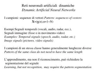
Reti neuronali artificiali dinamiche Dynamic Artificial Neural Networks I campioni: sequenze di vettori Pattern: sequences of vestors X=(x(n),n=1N) Esempi:Segnali temporali (vocali, audio, radar, ecc.), Segnali immagine (fisse o in movimento-video) Examples: Temporal signals (speech, audio, radar, etc.) Image signals (pictures, video signals) I campioni di un stessa classe hanno generalmente lunghezze diverse Pattern of the same class do not need to have the same length L’apprendimento, ma non il riconoscimento, può richiedere la segmentazione del segnale Learning, but not recognition, may require the pattern segmentation
- Tr x2 Tx r(t) t=10 x(t) t=0 x1 D(r,x) = |r(t)-x(t)|dt Distorsione temporale fra r(t) e quello di x(t); Time warping between r(t) and x(t) Tr= r(q(t)), ma q(t) non è definita ;but q(t) is not defined Gr(x) = min [ D(x,Tr); T C] C è l’insieme delle distorsioni q(t); C is the set of the time warping non significativa, not meaningful
Gr(x) = min [ |x(t)-Tr(t)| dt ; T C] - x(t) x(t) t r(t) t d0 T è l’ insieme dei ritardi d0 e delle distorsioni T is the set of delay d0 and time warping
B Richiamo al riconoscimento di segnali con HMM (Hidden Markov Model) Review of HMM for temporal signal recognition Principio di ottimalità (Bellman):“In un sistema a stati finiti la scelta ottimale attuale è indipendente dalle scelte ottimali precedenti” Optimality principle (Bellman):“The optimal local choice in a finite state system is independent of the preceeding optimal choices” PAA PBB PCC PAC PBA PCB S C E b) Catena di Markov Markov Chain
E=K B=k C S Sk,n 1n-1 n N Grafo degli stati; States Graph : Sk,n= (sk,n) ( k=1K e n=1N) Cott(S k,n) = DCk,n + argmin[C ott(S j,n-1)+t jk; j precedente di k; j preceding k] dove; where: DCk,n= (mk-xn)2sk2 tjk=-log(Pjk)
w1 Id1 c2 w2 Id2 c2+p2 w1 HMM/ w1 HMM/ w2 Id2 c2+p1 HMM/ w3 WLC WLC=Word Link Controller w3 Id2 c2+p3
n+1 x2 N X(n+1) n X(n) 2 X(N) X(2) a) 1 X(1) x1 x2 X(n),n b) X(2),2 x1 X(n+1),n+1 X(N),N X(1),1 n Traiettorie nello spazio delle caratteristiche Trajectories in the pattern space (a) e nello spazio caratteristiche-tempo and in the pattern-time space (b)
x(n) sj(n) wj sj(n) = wj x.(n-1) Connessione sinaptica dinamica elementare; BasicDynamic Synaptic Connection
j w4 1 + w3 w0 w1 w2 z-1 z-1 z-1 x(n) x(n-1) x(n-2) x(n-3) x.(n)=[x.(n),...,x.(n-P),1)]T; wT=[w0,...,wP+1,] x(n) sj(n) wj sj(n) = Sh wh.x.(n-h) = wj. x(n) Connessione sinaptica dinamica; Dynamic Synaptic Connection
j w4 sj(n) s(.) zj(n) + 1 w3 wj w0 w1 w2 z-1 z-1 z-1 xi(n) x(n-1) x(n-2) x(n-3) xi.(n)=[x.(n),...,x.(n-P),1)]T; wjT=[wj0,...,wj(P+1),] sj(n) = Sh wjh.xi.(n-h) = wj. xi(n) zj(n) =s(sj(n)) Nodo con connessione sinaptica dinamica (FIR non lineare) Node with dynamic connections (Non linear FIR)
Tipologie di RNA dinamiche Dynamic ANN typologies • 1) RNA a ritardo (Time-delay Neural Networks: TDNN) • 1.1) TDNN a ritardo concentrato (Focused TDNN) • 1.2) TDNN a ritardo distribuito (RNA convoluzionale) • Distributed TDNN (Convolutional TDNN) • 2) RNA ricorrenti; Recursive Dynamic ANN • 3) RNA spazio-temporali; Spatiotemporal ANN • 4) Reti di Hopfield; Hopfield Networks • 5) Memorie associative; Associative Memories • Apprendimento supervisionato; Supervised Learning • a epoche; epoch learning • in tempo reale; real time learning
y(n) RNA MLP, SOM T T T T T x(n) x(n-1) x(n-2) x(n-5) x(n-3) x(n-4) TDNN a ritardo concentrato; Focused TDNN
y(n+1) RNA MLP, SOM Strato d’ingresso Strato di contesto Input layer Context layer T T T T x(n) y(n) x(n-1) x(n-2) y(n-1) RNA ricorrente; Recursive Dynamic ANN
y(n) 1 j P segnale di Abilitazione; Start signal segnale di riconoscimento; End signal wj x(n) RETE SPAZIO-TEMPORALE ;Spatiotemporal Netwok Analogia topologica con le SOM e HMM Topological analogy with SOM and HMM
y(n) MLP zi yi(n) i 1 i M T T T x(n) x(n-Q) T Input memory of length Q; lunghezza del campo ricettivo; length of the receptive field: L= Q+1 Nodi dello strato nascosto; nodes of the hidden layer: M= Q+1 numero massimo di pesi diversi; maximum number of different weights: (Q+2)M; TDNN completamente connessa; Completed connected TDNN x(n) scalare o vettore; scalar or vector
yc strato di integrazione Integration layer strato di separazione delle classi Class separation layer T T T T T strato di convoluzione Convolution layer xn T T xn-2 xn-1 TDNN convoluzionale a pesi distribuiti; Distributed weights convolutional TDNN
y z1 z4 1 1 1 1 M w3 w1 w2 x(n) x(n-5) T T T T T Espansione temporale di una TDNN convoluzionale Time expansion of a convolutional TDNN Finenstra temporale e lunghezza del campo ricettivo: P=6; Time window and length of the receptive field: P= 6 numero di pesi; number of weights: Q=3 Nodi dello strato nascosto; number of nodes of the hidden layer: M= P-Q+1=4
Addestramento delle TDNN; Supervised learning of TDNN • TDNN a ritardo concentrato o convoluzionale • il segnale desiderato (classe) può essere presentato solo al termine dell’ epoca • la sequenza è segmentata, addestramento come MLP spaziale • addestramento a epoche • b) TDNN a ritardo concentrato • il segnale desiderato è presentato in ogni istante • processo stazionario, addestramento sequenziale come MLP • addestramento in tempo reale • Esempio: predittore non lineare • c) TDNN convoluzionale • il segnale desiderato è presentato in ogni istante • processo stazionario, addestramento sequenziale come MLP • addestramento in tempo reale
Addestramento delle TDNN; Supervised learning of TDNN a) Riconoscimento di segnali:Addestrameno a epoche con retropropagazione temporale dell’errore totale ed aggiornamento globale: n0<n<n1) Epochwise learning with total error back propagation and global updating: n0<n<n1 c) Predittori:Addestramento in tempo reale con errore locale ed aggiornamento in tempo reale; Realtime learning with local error and real time updating n0 n1 n
T=20ms (12x20ms = 0,24s) yb yd yg 3 8 16 T T T T T T T x(n) x(n-2) x(n-3) x(n-h) x(n-1) x(n-12) TDNN per il riconoscimento dei fonemi “b, d, g” ,Processi non stazioanri TDNN for “b,d,g” phonemes recognition, Npn stationary processes
1 3 1 8 x1(n) X(n) x16(n) Estenzione delle TDNN convoluzionali a segnali immagine Convolutional TDNN for image signals
y*(n)=x(n+1) _ e(n+1) + s(.) x’(n+1) w4 w3 w1 w2 z-1 z-1 z-1 x(n) x(n-1) x(n-2) x(n-3) Dwj= h e(n+1) s’(x(n+1)x(n-i) Predittore non lineare (processo stazionario); Addestramento in tempo reale Non linear predictor (stationary process);; realtime learning
y(n) = s(.) v1 v4 vi M zi(n) H1 w3 w1 w2 x(n) x(n-5) T T T T T d(n) = [y*(n)-y(n)]s’[v(n)] = e(n)s’[v(n)]; vi(n+1) = vi(n)+hd(n)zi(n); di(n-k)= d(n-k)vi(n)s’[zi(n-k)] i=14 (gradiente locale del nodo i di H1) wk(n+1) = wk(n) + 1/M[ hSidi(n-3)x(n-3-k-i+1)] per k=1,2,3 Addestramento in tempo reale di TDNN convoluzionale a uno strato Real time learning of a single hidden layer convolutional TDNN
z1(n) s(.) x1(n) w1 v1 x2(n) w2 z-1 z2(n) s(n) y(n) s(.) + s(.) z-1 v2 + z-1 z3(n) s(.) x3(n) w3 v3 Etot(W,v)= 1/2Sn (y*(n)-y(n))2 TDNN convoluzionale a due strati ( processi non stazionari) Two hidden layer convolutional TDNN (non stationary processes)
Processing equations Output layer (OL): y(n)=s[s(n)]; s(n)= Sjzj(n) Tvj OL dynamic synaptic weights:vj=[v0j,...,vPj,] Vector activity of node i of the hidden layer (HL): zj(n)=[1,zj(n),…,zj(n-P)]; zj(n)= s[sj(n)]; sj(n)= wiTxi(n); HL synaptic weights:wi=[w0i,...,wPi,] Input vectori: xi(n)=[1, xi(n),...,xi(n-P)]; Local gradient of the OL: d(n)= e(n)s’[s(n)]; vj(n+1)= vj(n)+hd(n)zj(n) Local gradients of the HL: Dj(n-Pj)=[dj(n),…, dj(n-P) ]; dj(n- Pj)= s’[sj(n- Pj)] Dj(n- Pj)Tvj Updating expression: wji(n+1)=wji(n)+hdi(n- Pj)Txi(n- Pj) Real time learning of a two hidden layers convolutional TDNN
T -1< wjj <1 wjj a) s(n) wij y(n) + s(s) xi(n) j yi(n) yj(n) yh(n) wji T wjj wji >> wij whi i j s(n) s(n) + + s(s) s(s) w1i wii wkj T b) w1j y1(n) wij yk(n) y1(n) Neuroni artificiali dinamici: retroazione locale (a) e con interazione (b) Dynamical Articial neurons: local feedback (a), interacting nodes (b)
y1 . 1 2 y2 u . y2(n+1) v12 1 v22 y1(n+1) 1 2 w11 w22 w21 w12 v11 v21 . T T y1(n) y2(n) u(n) RNA dinamica elementare; Basic Dynamic ANN (Flip-flop)
y(n+1) RNA MLP, SOM Strato d’ingresso Strato di contesto Input layer Context layer T T T T x(n) y(n) x(n-1) x(n-2) y(n-1) RNA ricorrente; Recursive Dynamic ANN
Metodi di addestramento per RNA dinamiche Riconoscimento di segnali Retropropagazione temporale a epoche (aggiornamento globale: n0<n<n1) Pattern recognitionBackpropagation through time (global learning n0<n<n1) b) Predizione Retropropagazione in tempo reale troncata a n-H ( aggiornamento con retropropagazione del solo errore istantaneo) Prediction Real time trunkated backpropagation at n-H (updating with the current error) c) Predizione Addestramento in tempo reale con l’errore locale Prediction Realtime updating using the current error n0 n1 n1 n0 H n n
y1(n-1) w1 w1 w1 w1 y1(n) y1(n+1) . . w12 w12 w12 . v1 v1 v1 u(n) u(n-1) u(n+1) v2 v2 w12 v2 w21 w21 w21 y2(n-1) w2 y2(n) w2 y2(n+1) w2 w2 s1(n)= u(n)v11+ v12+ y1(n-1)w1+y2(n-1)w12 s2(n)= u(n)v22+ v21+ y1(n-1)w21+y2(n-1)w2 y1(n)=s(s1(n)); y2(n)=s(s2(n)) E(v,w,n)= ½[ (y1*(n)-y1(n))2+ (y2*(n)-y2(n))2] Espansione temporale per l’ addestramento della rete Flip/flop Time expansion for the Flip/flop network updating
z-1 x(n) waj y(n) x(n+1) C z-1 wbj u(n) j x(n)T=[x(n), u(n)] con x(n) = (xj(n);j=1M wjT =[waj ,wbj], W=[waj ,wbj,j=1M] x(n+1)=s(WaTx(n)+WbTu(n)]=s[WTx(n)] y(n)=Cx(n) Struttura canonica della rete ricorrente Canonical structure of a recurrent ANN network
x(n-1) x(n) x(n+1) Wa Wa Wb Wb y(n+1) y(n) _ + _ + u(n) u(n+1) e(n) e(n+1) y*(n+1) y*(n) x(n)T=[x(n), u(n)]; x(n+1)=s(WaTx(n)+WbTu(n)]=s[WTx(n)]; Sviluppo temporale della struttura canonica per adddestramento con retropropagazione nel tempo Time expansion of the canonical structure for backpropagation through time learning
y(n) u(n) RNA x(n) x(n+1) T y*(n0 ) y*(n0 +1) y*(n1) y*(n1-2) y(n1) y(n0 +1) y(n1-2) y(n0) x(n1 -2) x(n0) RNA RNA RNA x(n0 +2) x(n1-1) x(n1) RNA x(n0 +1) u(n1) u(n1-1) u(n0) u(n0 +1) RNA ricorrente con sviluppo temporale da n0 a n1 Bachpropagation through from n0 to n1 for a Recursive ANN
x(n+1) x(n) RNA T y(n+1) y(n) u(n-1) u(n) u(n) u(n) y(n0 +2) y(n1-1) y(n1) y(n0 +1) x(n1 -2) x(n0) RNA RNA RNA x(n0 +2) x(n1-1) x(n1) RNA x(n0 +1) u(n1-1) u(n0) u(n0+1) u(n1-2) Espansione temporale di RNAD mista TDNN/recursiva; Time expansion of a mixed TDNN/recursive Dynamic ANN
e1eh=y*h- yheM yh O H2 H1 I s’(sh) 1 h M whj dh= ehs’(sh) Dwhj= h dh yj yj ej=S dh whj dj= ejs’(sj) s’(sj) 1 j MH2 wji Dwji = h dj yi ei=Sj dj wji di= ejs’(sj) yi s’(si) 1 i MH1 Dwik = h di xk wik x1xk xN 1 k N Rete di retropropagazione dell’ errore per RNA statiche Backpropagation network for feedforward ANN
e j(n)=y*(n)-y(n) e j(n0) e j(n1) dh(n) dj(n1) dh(n0+1) dh(n+1) n1 n n0 u(n1), x(n1-1) u(n), x(n-1) u(n0), x(n0-1) dj(n) = s’(s j(n))[ej(n) +ShwahjiTdh(n+1)]; dh(n1+1)=0 Dwaji = hSndj(n+1) xi(n); Dwbji = hSndj(n) ui(n); i,j= 1,…,N; n=n0+1,...,n1 Rete e formule per l’ addestramento a epoche con retropropagazione temporale di solito si impone solo y*(n1)=1 Backpropagation network and updating expressions for backpropagation through learning; usually only y*(n1)=1 is given
e j(n) dh(n-H+1) dh(n-H) dh(l) dh(n1) dh(l+1) n-H l n u(l), x(l-1) u(n-H), x(n-H-1) u(n), x(n-1) dj(n) = s’(sj(n))ej(n) dj(l) = s’(s j(l))[Shwhj(l)Tdh(l+1)]; e per n-H <l <n Dwaji(n)= hSldj(l) xi(1 -1); con n-H +1<l <n Dwbji(n)= hSldj(n) ui(1 -1); con n-H +1<l <n Addestramento in tempo reale e retropropagazione temporale troncata Realtime updating with truncated temporal backpropagation
y(n) w v u(n) x(n)=y(n-1) T y(n)=s[s(n)]; e(n)=y*(n)-y(n); s(n)=w(n) u(n)+v(n)x(n); Stato della rete; network state: x(n) = y(n-1) Aggiornamento del peso d’ingresso; input weight updating: Dw(n) = h e(n) dy(n)/dw = h e(n) s’(s(n) ds(n)/dw = hd(n) u(n) Aggiornamento del peso di contesto; context weight updating: Dv(n) = h e(n) dy(n)/dv= he(n) s’(s(n)).ds(n)/dv = hd(n)[x(n)+v(n) dx(n)/dv] dx(n)/dv = dy(n-1)/dv =s’[s(n-1)][x(n-1)+v(n-1) dx(n-1)/dv] condizione iniziale; initial condition: dx(1)/dv = k Addestramento in tempo reale: Percettrone ricorrente Realtime learning: Recursive Perceptron
z-1 x(n) waj y(n) x(n+1) C z-1 j wbj u(n) x(n)T=[x(n), u(n)] con x(n) = (xj(n);j=1M wjT =[waj ,wbj], W=[waj ,wbj,j=1M] x(n+1)=s(WaTx(n)+WbTu(n)]=s[WTx(n)] y(n)=Cx(n) Struttura canonica della rete ricorrente Canonical structure of a recurrent ANN network
Addestramento in temporeale (Vedi: S. Haykin “Neural Networks” Cap. 15.8) E(W,n)=1/2e(n)Te(n); e(n)=y*(n)-y(n)= y*(n)-Cx(n) dE(W,n)/dwj=[de(W,n)/dwj]Te(n) = -e(n)TCdx(n)/dwj aggiornamento dei pesi di contesto; updating of the weights of the context layer: Dwj(n)= -h dE(W,n)/dwj= he(n)TCdx(n)/dwj Matrice delle derivate dello stato; matrix of the state derivatives: Lj(n) = dx(n)/dwj=dx(n)/ds(n).[ds(n)/dwj] Dwj(n) = he(n)T CLj(n)
Calcolo di; computation of: Lj(n) Lj(n) = dx(n)/dwj=dx(n)/ds(n).[ds(n)/dwj] x(n+1) = (s(w1Tx(n)),...,s(wjTx(n)),...,s(wqTx(n)) s(n+1)=W(n)Tx(n) = wa(n)Tx(n)+wbTU(n-1) derivando si ha la recursione; recursive expression: Lj(n)= F(n-1)[Wa(n-1)Lj(n-1)+Uj(n-1)] con Lj(0)=0 Dove; where: F(n)= diag[s’(w1Tx(n)),...,s’(wjTx(n)),...,s’(wqTx(n)] Uj(n)T=[0,..., x(n)T,...,0] alla j-esima riga
yi(n) 0 1 2 4 3 wi w3 w4 w1 Conness. con ritardo Reset u(n) W3 u(n) x2 W4 W2 W1 x1 Rete spazio temporale: struttura globale analoga alle SOM e HMM Spatiotemporal network: structure similar to SOM and HMM
sK si si-1 s1 vi vi vi wi vi-1,i vi-1,i vi-1,i u(1) u(n-1) u(n) u(n+1) u(N) Addestramento ad epoche della RNA spazio-temporale: vedi HMM Backpropagation through time of a spatiotemporal ANN
y(n) C z-1 wi(n) vi (n) i vi-1,i (n) xi(n+1) u(n) Addestramento in tempo reale della RNA spazio-temporaleRealtime learning of a spatiotemporal ANN
yN(n) y0(n)=1 y1(n) yi(n) yN-1(n) yi-1(n) 1 2 i K w2 wi wK w1 a) x(n) si(n) yi-1(n-1) yi(n) yi-1(n) + T u(si-Si) ai x(n) d(.,wi) u(Ri-d) b) T i (a) RNA spazio-temporale con attivazione in cascata; Spatiotemporal ANN with cascade activation; (b) nodo; node. Addestramento non supervisionato (metodo di Hecht-Nielsen) Unsupervised learning (Hecht-Nielsen Method)
w2 Classificatore statico Static classifier x2 SOM w1 x x x Classificatore Dinamico Dynamic classifier w(n) w2 o RNA Hopfield x w2 x w3 n >0 n=0 x1 w(0)=x RNA dinamiche per il riconoscimento di campioni statici Dynamic ANN for static pattern recognition
w1(n) w3(n) w2(n) w3(0) = x3 Tij i w2(0) = x2 w1(0) = x1 j Tij =Tji n> 0 n =0 Rete di Hopfield; Hopfield Network