Download
1 / 37
380 likes | 532 Views
TeV Cosmic-ray Anisotropy & Tibet Yangbajing Observatory. Qu Xiaobo. Institute of High Energy Physics. Yangbajing Observatory. ARGO Hall. Tibet AS array. The Tibet Air shower Array. Located at an elevation of 4300 m (Yangbajing , China) Atmospheric depth 606 g/cm 2

E N D
TeV Cosmic-ray Anisotropy & Tibet Yangbajing Observatory Qu Xiaobo Institute of High Energy Physics
Yangbajing Observatory ARGO Hall Tibet AS array
The Tibet Air shower Array • Located at an elevation of 4300 m (Yangbajing , China) • Atmospheric depth 606g/cm2 • Wide field of view (Dec. -15º,75º ) • High duty cycle (>90%) • Angular resolution (~0.90) Advantage----measurement of Cosmic ray Large scale anisotropy
OUTLINE • Large scale anisotropy in sidereal time • Energy dependence • Time evolution • Models • Compton-Getting effect • Solar time anisotropy • Periodicity • Summary
Sidereal time anisotropy Energy dependence Harmonic analysis decrease increase independent “East-west”(E-W) subtraction method Amenomori, APJ, 2005
Anisotropy expected by CR production and propagation Diffusion model: The amplitude of anisotropy (R – rigidity) (δ ~ 0.3-0.6 ) increase with the energy! • Random character of SN explosions; • Mixed primary mass composition; • Possible effect of the single source; • 4. The Galactic Halo; A. D. Erlykin, A. W. Wolfendale, Astropart. Phys. 25, 183(2006) Important probe, discover CR origin, study CR propagation.
Sidereal time anisotropy Tail-In max. shifts earlier in the south Loss-Cone Tail-In Loss-Cone Tail-In Hall et al. (JGR, 104, 1999) Tail-in Structure analysisNFJ model Loss-cone Gaussian analysis Hall et al. (JGR, 103, 1998)
Two dimension analysis method Zenith On-source Off-source Off-source ——Global fitting method Zenith belt Equal
Tibet measurement in two dimensions The CR anisotropy is fairly stable in two samples. Three Componets: I--------Tail-in; II-------Loss-cone III------Cygnus region; <<Anisotropy and Corotation of Galactic Cosmic Rays >> M. Amenomori et al., Science, 314 429 (2006)
Large scale anisotropy in two dimension Milagro Super-Kamiokande-I Also by ARGO, Icecube
Energy dependence Celestial Cosmic Ray intensity map in five energy range 4 TeV <12TeV Energy independent >12TeV Fade away 6.2 TeV 12 TeV 50 TeV “Tail-in” effect exists in 50TeV, rule out the solar causation. 300 TeV
Energy dependence 0.7TeV 1.5TeV 3.9TeV Sidereal time anisotropy by ARGO Median energy Consistent with the 1D observations, finer structure in 2D <<Observation of TeV cosmic ray anisotropy by the ARGO-YBJ experiment>> ICRC0814,2009
Temporal Variations Sidereal time anisotropy in 9 Phases (1999-2008) Improved analysis method, more statistic. Stable Insensitive to solar activities <<On Temporal Variations of the Multi-TeV Cosmic Ray Anisotropy Using the Tibet III Air Shower Array>>, M. Amenomori et al., ApJ 711, 119 (2010)
Temporal Variations Time Evolution of the Sidereal Anisotropy Matsushiro Observation No steady increase Tibet Observation 2000-2007 Milagro observation The fundamental harmonic increase in amplitude with time. 1999-2008
Sidereal time anisotropy in two hemisphere Tibet III Icecube
Sidereal time anisotropy in Galactic coordinate Tibet III Icecube Excess Cosmic ray flows in three directions Inward flows Outward flows Electrically neutral state X.B.Qu et al., arXiv:1101.5273
Magnetic field induced by Cosmic ray flows Extend the anisotropy image observed in the solar vicinity to the whole Galaxy. Biot-Savart Law A0 dynamo model J.L. Han,1997 • Magnetic Field Structure, Consistent • The extension of the local anisotropy to the whole Galaxy is reasonable. X.B.Qu et al., arXiv:1101.5273
Alternative Model of the Sidereal time anisotropy Global +Midscale Anisotropy uni-directional flow +bi-directional flow Local interstellar magnetic field Two intensity enhancements along a Hydrogen Deflection Plane In,m(MA) Hydrogen Deflection Plane In,m(GA) In,m Residual anisotropy after subtracting In,m(GA) Residual anisotropy after subtracting In,m Amenomori, M., et al. 2010, Astrophys. Space Sci. Trans., 6, 49
Alternative Model of the Sidereal time anisotropy LIMC (Local Interstellar Magnetic Cloud) model Local Interstellar Cloud, egg-shaped cloud, 93 pc3. Cosmic ray density (n) lower inside LIC than outside, adiabatic expansion ⊥Perpendicular ∥Parallel uni-directional flow (UDF) ⊥ bi-directional flow (BDF) ∥ LISMF
j E-a 8 Δ I < I > v c = ( a+ 2 ) cos q Known origin of large scale anisotropy——Compton-Getting Effect Due to the solar motion around galactic center V=220km/s,a = 2.7 Expected dipole effect We could observe A.H. Compton and I.A. Getting, Phys. Rev. 47, 817(1935)
Celestial Cosmic Ray intensity map for 300 TeV Expected Expected Amp= 0. 16% The statistic error 0. 026%, ~5σ rule out the Compton-Getting effect. These results have an implication that cosmic rays in this energy range is still strongly deflected and randomized by the Galactic magnetic field in the local environment.
Known origin of large scale anisotropy—— Compton-Getting effect ΔI < I > v c = ( a+ 2 ) cos q Due to terrestrial orbital motion around the Sun Differential E spectrum : j E-a 8 V=30km/s,a = 2.7 D.J. Cutler, D.E. Groom, Nature 322, L434 (1986) The amplitude is ~0.04%
Tibet measurement in solar time I ——Compton-Getting effect (12TeV) The solar time anisotropy is stable in two intervals with different solar activity The 1D modulation (solid line) is consistent with the expected one (dash line)。
Tibet measurement in solar time II ——Additional effect (4TeV) Preliminary With the compton-getting effect subtracted. The amplitude ~0.04%.
Periodicity search in 3 energy ranges • Sidereal semi-diurnal Solar diurnal. Compton-Getting effect • Sidereal-diurnal <<Observation of Periodic Variation of Cosmic Ray intensity with the Tibet III Air Shower Array>>, A.-F. Li Nuclear Physics B,, 529, 2008.
Summary • Yangbajing Observatory successfully observed the Cosmic ray anisotropy.(0.7TeV-300TeV) • Energy dependence, time evolution, Periodicity analysis of the anisotropy • In the sidereal time frame, revealing finer details of the anisotropies components “tail-in” and “loss-cone” and “Cygnus” region direction. Models given. origin??? • In the solar time frame, Compton-Getting effect is observed in 12TeV, An additional modulation appears to exist in case of low energy.
Thanks for your attention! 中意ARGO实验大厅 中日AS探测阵列
Anisotropy Observations in other periods Anti sidereal time Ext-sidereal time No signal is expected, the amplitude observed is within statistic error.
银河宇宙线在磁场中传播 Cygnus方向 银河系磁场强度为3uG时 回旋半径 3TeV对应0.001pc (200AU) 带电粒子在传播过程中受磁场影响而偏离其原本方向.星际磁场就像一个搅拌机,将宇宙线粒子搅拌得各向同性.
Sidereal time anisotropy components ——NFJ model
Loss-Cone Tail-In max. shifts earlier in the south Tail-In Nagashima, Fujimoto, Jacklyn (JGR, 103, 1998) Hall et al. (JGR, 103, 1998)
Sidereal time anisotropy One-dimensional observation
太阳时各向异性 宇宙线及大尺度各向异性 存在截止刚度 ,经测量 随太阳 活动有11年的周期变化,活动极小时,低至几GV,极大时,可达200GV 最近观测发现,600GV宇宙线太阳时各向异性仍受到太阳活动的调制;Tibet ASγ在4TeV处观测到超出CG效应的太阳时各向异性,高能处与预期CG效应一致 低能处比较明显,随刚度幂律分布
Medium scale anisotropy Milagro ARGO Tibet-III
Large scale anisotropy Milagro Tibet-III