Download
1 / 19
200 likes | 358 Views
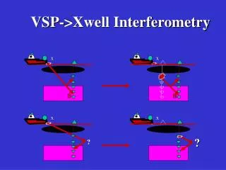
x. x. B. B. x. x. ?. VSP->Xwell Interferometry. ?. 3x3 Classification Matrix. SSP. VSP. SWP. SSP. SSP. SSP. SSP. VSP. SSP. SWP. VSP. VSP. SSP. VSP. VSP. VSP. SWP. SSP. SWP. SWP. SWP. VSP. SWP. SWP. Xwell. Xwell. Xwell. SSP. Xwell. VSP. Xwell. x. x. x.

E N D
x x B B x x ? VSP->Xwell Interferometry ?
3x3 Classification Matrix SSP VSP SWP SSP SSP SSP SSP VSP SSP SWP VSP VSP SSP VSP VSP VSP SWP SSP SWP SWP SWP VSP SWP SWP Xwell Xwell Xwell SSP Xwell VSP Xwell
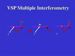
x x x VSP Experiment A A A B B B G(A|x)* G(B|x) G(A|x) o Model based Needs V(x) around well x B VSP->Xwell Transform
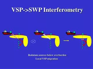
VSP Experiment x B Motivation Problem: Overburden+statics defocus VSP migration Solution: VSP -> Xwell Transform Redatum sources below overburden Local VSP migration
(a) VSP data: P(g|s)=T(g|s)+R(g|s) s g R(g|s) x (b) Backward reflection (c) Backward transmission T(g|s) s R(x|s)= G(x|g)*R(g|s) T(x|s)= G(x|g)*T(g|s) g g g R(g|s) x x x T(g|s) R(g|s) (d) Crosscorrelation m(x)= R(x|s)T(x|s)* g g g Key Idea of Local RTM s Local VSP Green’s function Theory
Numerical Results 1. Synthetic VSP (Jinahua Yu) 2. Synthetic VSP (Xiang Xu) 3. GOM VSP
Walkaway VSP 0 km Source number: 100 Shot interval: 10 m Receiver number: 91 Receiver interval: 10 m Depth of the first receiver: 950 m Depth of the last receiver: 1850 m Temporal interval: 0.001 s 2 km 0 km 3 km
950 Depth (m) 1950 X (m) X (m) 1000 1400 1000 1400 Local VSP Migration Image No Overburden velocity needed No need to know source location or excitation time
Limitations Rotated Pyramid vs Pyramid Traditional VSP Local VSP D L
Numerical Results 1. Synthetic VSP (Jinahua Yu) 2. Synthetic VSP (Xiang Xu) 3. GOM VSP
Sigsbee P-wave Velocity Model m/s 0 4500 279 shots Depth (km) 150 receivers 1500 9.2 Offset (km) 12.5 -12.5
Local Reverse Time Migration Results Migration image True model 4.6 f Depth (km) 9.2 -3 Offset (km) 3
Numerical Results 1. Synthetic VSP (Jinahua Yu) 2. Synthetic VSP (Xiang Xu) 3. GOM VSP
GOM VSP Well and Source Location Source @150 m offset 0 Depth (m) 2800 m Salt 82 receivers 3200 m 4878 Offset (m) 1829 0
Velocity Profile S Wave P Wave 0 Incorrect velocity model Depth (m) P-to-S ratio = 2.7 2800 m Salt P-to-S ratio = 1.6 3200 m 4500 0 5000 0 5000 Velocity (m/s) Velocity (m/s)
Z-Component VSP Data 2652 Reflected P Salt Depth (m) Reverberations Direct P 3887 1.2 3.0 Traveltime (s)
X-Component VSP Data 2652 Reflected P Salt Depth (m) Direct S Reverberations Direct P 3887 1.2 3.0 Traveltime (s)
Local Reverse Time Migration Result 3.3 (2) 39 receivers (1) Depth (km) (3) 3.9 reflectivity 0 Offset (m) 100 (1) specular zone, (2) diffraction zone, (3) unreliable zone
Conclusions • VSP->XWell transform alternative to VSP_>SWP and VSP->SSP transforms • Source statics eliminated, no need to know src. Location or excitation time • Local v(x) needed, overcomes defocusing due to overburden • Not battle-field tested, needs decon probably, weird resolution characteristics