Pedagogical Introduction

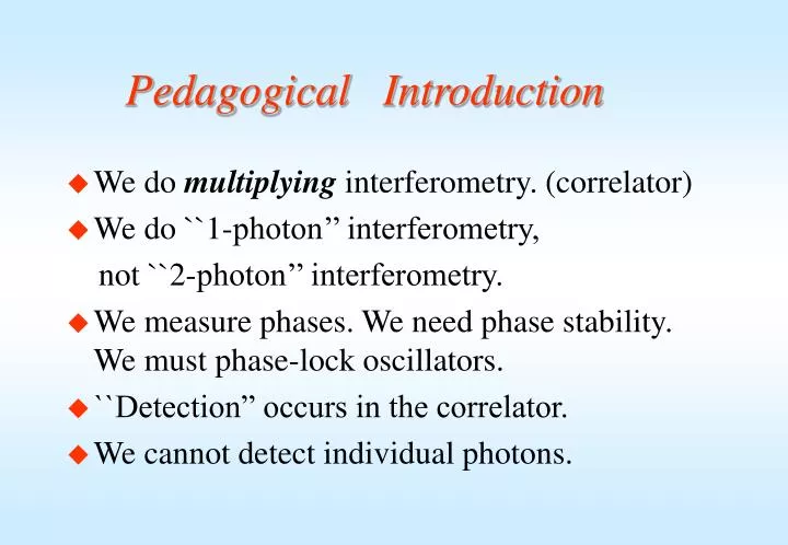
1. Pedagogical Introduction • We do multiplying interferometry. (correlator) • We do ``1-photon’’ interferometry, not ``2-photon’’ interferometry. • We measure phases. We need phase stability. We must phase-lock oscillators. • ``Detection” occurs in the correlator. • We cannot detect individual photons.

2. : 2 kinds.We do this. We don’t do this. (One-photon interferometry)

3. We REALLY do ``one-photon’’ interferometry: • Example: • Typical flux density at 3mm~ 1 mJy = 1.3E-7 photons / sec / m2 / Hz. • 2 x 15-m dishes => collecting area = 230 m2. • In 1-MHz band, power to 2 dishes = 30 photons/sec. • For clock rate of 320 MHz, sample time = 3.1 nsec. • So we record ~10 million samples before getting one photon from the sky. • Is this OK ? Can we get interference?

4. ``1-photon’’ interference: A student’s experiment in 1909. • Geoffrey Taylor (student of J.J. Thompson). • NB: Max Planck’s theory of quanta (1900). • Taylor 1909, Proc. Camb. Phil. Soc., 15, 114

5. Taylor’s physics experiment, built at home: Geoffrey Taylor’s 1909 prototype of the Plateau de Bure interferometer. Left: strong, many-photon light. Right: 1-photon at a time. (no difference).

6. ``A photon only interferes with itself’’. --- Dirac (1932) Dirac got this by pure thought. Taylor’s paper was long-forgotten. (In fact, only ``probabilty amplitudes’’ interfere, not the photons). But what about the 2-path, 2-dectector interferometer? Suppose you send it only ``one photon’’ at a time? Try it in the lab. Detectors

7. One beam splitter: 2 paths, 2 detectors post-detection correlation; try one photon: get zero correlation ! • Conclusions: • Photon not a wave. • Can identify path. • No interference. • NOT WHAT WE DO. • What saves us? Detector Detector Beam splitter Correlation vs. photon number 1 photon 2 photons Grangier, Roger, Aspect (1986)

8. Add a 2nd beam-splitter: (Mach-Zehnder) now have 2 paths, correlate at end, just like our mm interferometer.

9. M-Z like Plateau de Bure interferometer: 2 paths, correlate at end. Antenna 1 path Antenna 2 path Single-photon input

10. One photon input to M-Z: fringes as function of path delay. Grangier, Roger, Aspect, 1986, Europhys. Lett., 1, 173

11. Hanbury Brown’s radio interferometer of 1952. Almost right for us. BUT WE DON’T DO THIS : Our ``detector’’ is here :  ( the Correlator ) Note: Cables not necessary. Hanbury-Brown used WiFi (in 1952 !!).

12. Enloe & Rodda 1965, Proc. IRE, 55, 166 Bell Labs, Holmdel, N.J. Lasers on shock-mounted concrete bloc, in a concrete vault. Importance of phase-locking: Can lasers interfere?

13. Can two lasers interfere? Yes, if you phase-lock. This is Young’s 2-slit experiment, without the slits !!

14. ``One photon comes from two lasers !! ’’ Now Repeat Taylor’s experiment of 1909. Reduce flux to 1-photon. Just like PdB mm –interferometer: 2 phased paths, 1-photon-at-a-time. The interference pattern will still build up. ( ``A photon only interferes with itself.” )

15. Another way to think of it.Loudon,Quantum Theory of Light, in agreement with W.E. Lamb’s ``Anti-photon’’ critique. . • A ``photon’’ is not a globule of light, traveling like a bullet through the interferometer. • Regard the interferometer as a tuned, (phase-locked) resonant cavity, that allows traveling-wave modes. • A 1- photon excitation of a mode is distrubuted over the entire interferometer, including the two internal paths.

16. Yet another way to think of it: • Think of the two antennas (2 slits) as a filter. • The filter takes one QM state and gives you another (like an ``operator’’ on a Hilbert space). • The filter convolves 2 delta-functions of position with the original state to give you a different state on the other side of the 2 slits. • In contrast, you give the detector a QM state, and it gives you back a number. • Filters and detectors are very different things.

17. The ``quantum limit’’ for receivers is irrelevant for interferometry. • The receiver ``quantum limit’’ means k TR = h . • So the receiver steadily emits 1 photon in (1/) sec. • In a 1-MHz band, a receiver at the ``quantum limit’’ emits 106 photons /sec. • But in a 1-Mhz band, 2 x 15m antennas looking at a 1-mJy source at 3mm collect only 30 photons/sec. • So there is no way we can recognize that an individual photon comes from the sky.

18. Question in an interferometry course: Suppose we could detect an individual photon (e.g. on a hard disk at one antenna of the Plateau de Bure interferometer). Then how can we get interference?

19. The usual way to think of it. The usual diagram of radio interferometry is a space-space diagram. It’s a snapshot at an instant in time.

20. Usual diagram of Radio interferometry • An interferometers measures coherence in the electric field between pairs of points (baselines). Direction to source wavefront ct Bsin  B T2 T1 (courtesy Ray Norris) Correlator • Incoming signals are corrected for geometric delay t and multiplied to yield a complex visibility, V =|V|ei, which has an amplitude and phase.

21. Another way: a space-time diagram: 1 Photon in from sky to interferometer which is at rest in space, moving only in time (vertical straight line).

22. Change the Lorentz frame: One photon in, two photons out. One is an induced photon, One is spontaneous emission. Which is which? No way to tell. Hence we cannot identify the path. Hence we can do inteferometry.

23. Basic Concepts • An interferometer measures coherence in the electric field between pairs of points (baselines). Direction to source wavefront ct Bsin  B T2 T1 (courtesy Ray Norris) Correlator • Because of the geometric path difference ct, the incoming wavefront arrives at each antenna at a different phase.

24. Aperture Synthesis • As the source moves across the sky (due to Earth’s rotation), the baseline vector traces part of an ellipse in the (u,v) plane. B sin  = (u2 + v2)1/2 v (kl) Bsin  T2  u (kl) B T1 T2 T1 • Actually we obtain data at both (u,v) and (-u,-v) simultaneously, since the two antennas are interchangeable. Ellipse completed in 12h, not 24!