Solving Multivariate Nonlinear Polynomial Systems
Solving Multivariate Nonlinear Polynomial Systems. Computer Aided Geometric Design (236716) Spring 2006. Massarwi Fady. References.

Solving Multivariate Nonlinear Polynomial Systems
E N D
Presentation Transcript
Solving Multivariate Nonlinear Polynomial Systems Computer Aided Geometric Design (236716) Spring 2006 Massarwi Fady
References • "Computation of the solutions of nonlinear polynomial systems", by E. C. Sherbrooke and N. M. patrikalakis. Computer Aided Geometric Design, Vol 10, No 5, pp 379-405, 1993 • "Geometric Constraint Solver using Multivariate Rational Spline Functions", by G. Elber and M. S. Kim. The Sixth ACM/IEEE Symposium on Solid Modeling and Applications, Ann Arbor, Michigan, pp 1-10, June 2001. • "Subdivision methods for solving polynomial equations", by B. Mourrain and J. P. Pavone, Technical Report 5658, Inria, Sophia-Antipolis, 2005.
Problem definition • Given a set of n rational polynomial functions of m variables: • And m dimensional box • Find solution such that
Definitions • Multi Index I is an ordered m-tuple of non-negative integers • Example : if M=(1,1) then • Bernstein i’th polynomial of degree m : • Bernstein basis function determined by multi index I and bounded by multi index M is defined by:
Problem definition • Since each function f is polynomial it can be represented by a basis change in Bernstein basis • Define the graph F of the function f as :
Problem definition • Since • We can write • And write the graph F of each function as : • The set of V are the control points of F, this representation is much powerful and allows to use different properties of Bernstein basis ( like convex hull property ) • u is a solution to the polynomial system if the point (u,0) contained in all the graphs Fi
Subdivision-based techniques • Numerical methods to find areas (box) where a single root ( solution ) could be found • In each step, If the current box dimensions are larger than some tolerance split it into two boxes and search in each of them recursively. • Advantages: • Speed • Stability • Simple • Disadvantages: • Designed for zero dimensional solution set -- No guarantee that all the roots are found • Doesn’t supply information on the root multiplicity
Subdivision-based techniques • We will review The following: • Subdivision while restricting the search domain • PP ( projection polyhedron ) , LP (linear programming ) - ( Sherbrooke & Patrikalakis) • Subdivision with numerical improvements ( Elber & Kim ) • Usage examples • Further improvements ( Mourrain & Pavoni)
Subdivision with domain restriction • Representing the graph of each function in the Bernstein basis allows us to use the convex hull property – The graph is contained in the convex hull of its coefficients ( vi ) • If there is a solution for all the equations then the point should be contained in all the graphs, thus in the intersection of the convex hulls of the graphs coefficients
Algorithm • Assume domain box is B = [0,1]n • Form the convex hulls of all Fk and intersect them with one another and with the hperplane un+1=0, call the intersection set A, if A is smaller than a tolerance stop. • A=A’X{0}, find a box B’=[a1,b1] X[a2,b2] X….. X[an,bn] that encloses A’ • If B’ is not singificantly smaller than [0,1]n, split B into equally sizes sub domains and work with each sub domain separately • For each k, define new function f’k by • Can be computed by De Casteljau multivariate subdivision • Update B with B’ and continue from step 2
Algorithm ( cont’d) • Step 2 contains two heavy operations • Computing the convex hull in dimension n • Intersecting all the convex hulls • Actually what we need is the bounding box of the intersection of the convex hulls, this can be achieved in different simple way
Algorithm ( updated ) • (1) -Start with initial search box • (2) - Perform transformation that brings the search box to [0,1]n • (3) - Find a sub box of [0,1]n which contains the roots • (4) - Use the reverse of the transformation used in step 2 to determine if the sub box is too small in Rn, if yes there is a root there and report for the mid point of the box. • (5) - if the dimensions of the box is close to 1 , split the box into two parts in each dimension. • (6) - Go back to step 2, once for each box.
Finding the Bounding Box of the intersection of the CHs • Projected Polyhedron ( PP ) • Find the width of the bounding box in each dimension by projecting it in that dimension • For dimension j: • For each graph Fk project each of it’s control points u to (uj,un+1) ( call it x-y plane ) • Form the convex hull in 2d of the projected points • Return as [aj,bj] the intersection of the convex hull with the X axis in the projection plane ( between 0 and 1 for all the graphs ). • Finally the bounding box will be • B = [a1,b1]X [a2,b2]X…… X[an,bn]
Finding the Bounding Box of the intersection of the CHs • Linear Programming ( LP ) • minimization function - If we look at the i’th coordinate of the points lying in the feasible area , what is the smallest ( ai ), and what is the biggest ( bi ) • Constrains – for each point x in the feasible area , it must satisfy • xn+1 =0 • For each k between 1 and n , x is contained in the convex hull of Vk (the control points of Fk)
Linear Programming • Formally • Minimization functions: • Constrains • Each point u is in the convex hull
Linear Programming • The unknowns are the coefficients • The number of the unknowns is
Analysis • The algorithm terminates • The subdivision factor (p) < 1 => • Linear convergence in the PP method • Quadratic convergence in the LP method
Linear convergence in the PP method • Given a box B=[a1,b1]x[a2,b2]x…x[an,bn] which contains one and only one simple root x0 of a system of polynomials f0,k:[0,1]nR where k ranges from 1 to n. let fk represent the subdivision of f0,k over B. Let the new box after executing one step of the PP method, denoted by B’=[a’1,b’1]x[a’2,b’2]x…x[a’n,b’n]. Let j be an integer between 1 and n, and let ( the lengths of the j’th side ) then
Linear convergence in the PP method - Proof • Let and g(u) is the linear approximation of f, • Then the following holds :
Linear convergence in the PP method - Proof • The projected control points of the graphs of the functions f, g ( (u,f(u)), (u,g(u)) ), are separated by vertical distances no more than • The projection of G on the (uj,un+1) plane is planar region ( because G is linear approximation ). For a fixed uj, the difference between the maximum y-coordinate and minimum y coordinate of this region is given by: • This is obtained from g(x1)-g(x0), where x0={0,0,…,xj,0,0,…,0} , x1={1,1,…,xj,1,1,…,1}
Linear convergence in the PP method - Proof • Then we can say that the whole projected control points of F are enclosed by two parallel lines that has a distance of from each other and slope of • Then if we look at the intersection of these two lines with the x axis ( between 0 and 1), the distance between the intersections ( which is translated to the box dimension later ) is :
Linear convergence in the PP method - Proof • Since • But we do scaling to transform the box to Rn, by scaling by , and this is the new box we work with so the new box dimension is
Quadratic convergence in the LP method • Given a box B=[a1,b1]x[a2,b2]x…x[an,bn] which contains one and only one root u0 of a system of polynomials f0,k:[0,1]nR where k ranges from 1 to n. let fk represent the subdivision of f0,k over B. After executing one step of the LP method, and let the new box denoted by B’=[a’1,b’1]x[a’2,b’2]x…x[a’n,b’n]. Define . There exists a neighborhood U of u0 and a depending only on U such that if and Let Then
Quadratic convergence in the LP method-proof • The linearization of the n fk is • Lets denote by p={p1,p2,…,pn,0} the intersection ( in Rn+1 ) of all gk (k=1..n) with xn+1=0 ( i.e g1=g2=…=gn=xn+1=0 ) ( such a point exists since the Jacobian matrix is not zero ) • Pick a point q=(q0,q1,…,qn,0) that lies in the intersection of F1, F2,…, Fn with hyperplane xn+1=0 • We know that • Substitute (q0, q1,…, qn) for x, since all fk are zero there, then
Quadratic convergence in the LP method-proof • letting rk=gk(q1,q2,…,qn), then there exists n points rk=(q1,q2,…,qn,rk) such that rklies on linear approximation of Fk, • For point p we know that • Subtracting * and **, and define we get
Quadratic convergence in the LP method-proof • By Cramer’s rule we get ( assuming the Jacobian matrix is non singular ) that where J is the Jacobian matrix , and Jk is the Jacobian matrix after exchanging k’th column with the column vector (r1,r2,…,rn)T • Since then and since we get • Then
Quadratic convergence in the LP method-proof • q is chosen arbitrary and its distance from other fixed point ( p ) is , then the distance between two points in the bounding box we want is also • Then the length of each side of the bounding box is also • The real size then ( in Rn ) is multiplied by factor of the bounding box ,then the dimensions of the new bounding box is • This hold for all K , then
Subdivision with numerical improvements • Subdivide the multivariate functions bounded within a certain resolution • Using the convex hull property if for a constrain Fi all the control points have the same sign then it won’t have a roots. • For each cell with dimensions lower than the wanted resolution report for a root ( center of the cell ) • Subdivision is terminated when it is known that there is an isolated root in the domain, in this case Newton-Raphson iterations is applied ( with quadratic convergence ) • If the zero set has a dimension larger than 0, then fit a multivariate surface to the set of the discrete points found by means of least squares ( minimizing the L2 norm )
Numerical improvement of the solution • for a given approximated solution u0 found , such that for each constrain Fi(u0)~0, using first order approximation, each graph Fi constrains the solution to be on the hyperplane which is defined in the point u0 as following : • Consider the normal to the surface Fi(u) at the point u0 : • Then the hyper plane at the point u0 is defined as
Numerical improvement of the solution • There are m such planes , and with the additional constraint that the component um+1=0, we end with n+1 linear equations( with m+1 variables) • If n=m then the system is full constrained and there is one solution • Otherwise if n < m a least square solution is found in an L2-norm ( finds the closest solution to u0 from the possible solutions set)
Uniqueness of a solution • If it is known that there is a single solution then it would be better to stop the subdivision and move to more efficient numerical procedure for root finding. • Definitions: • Cone: • normal cone of hypersurface Fi : set of all possible normal vectors on Fi . • Complementary (Tangent) cone:
Uniqueness of a solution • Theorm: • Given m implicit hypersurfaces Fi(u)=0 . i=1,…m in Rm, there is at most one common solution if • Proof: • Consider u0 (in Rm) is a common solution of the m equations Fi(u)=0. Consider , from the relation we have
Examples • Ray-Traps • Definition: • Given a set of n planar curves, it’s ray-trap of length n is a set of n points {Pi=Ci(ui)} such that a ray bouncing from Pi towards P(i+1)mod n will be reflected toward P(i+2)mod n • The incoming ray from Pi-1 and the outgoing ray towards Pi+1 should form an identical angle with the normal of Ci at Pi • This can be written as:
Examples • Surface-Surface Bisectors • Let S1(u,v) and S2(u,v) be two regular rational surfaces in R3 The points B=(x,y,z) on the bisector surface of S1 and S2 must satisfy the following constraints
Examples-Bisectors • Let • Then we can choose and the problem is reduced to
Examples-Bisectors • 4 variables with 2 equations – under constrained problem • Can fit a bi-variate surface to discrete points sampled on the solution space.
Further improvements • Preconditioning • Transformation of the system f=0 into equivalent system Mf=0 where M is nXn non singular matrix • global transformation • Useful when two or more functions have closed graphs on the domain, aims to increase the distance between them • The distance between two graphs is not trivial, so it is replaced by the distance between the vectors of the Bernstein basis coefficients • Local straightening: • Interesting situation of reduction is when the zero-set of the function fi are orthogonal to the xi direction
Preconditioning-global transformation • If then define the inner product between functions • Let and let E be a matrix of unitary eigenvectors of Q. Then f’=Ef is a system of polynomials which are orthogonal for the inner product above. • Proof:
Preconditioning- Local straightening • Local straightening • A better domain reduction can be done when the zero level of the functions fi are orthogonal to the xi axis. • This can be done by transforming the system f=0 in order to be closed to case (b). Transform locally the system into a system Jf-1(u0)f, where Jf is the Jacobian matrix of f at the point u0
Questions ??? Thanks
Further improvements - Reduction • For a function f and j=1,…,n let • Then • For any root u=(u1, u2 ,…, un) of the equation f(u)=0, we have where • t1/t2 is either a root of mj(f;uj)=0 or Mj(f;uj)=0 in [aj,bj] or aj/bj if mj(f;uj)=0/ Mj(f;uj)=0 has no roots in [aj,bj] • mj(f;uj)<=0<=Mj(f;uj)
Further improvements • Reduction • Similar to the PP ( projected Polyhedron ) , reduce the domain of search • PP is based on the convex hull property • The improvement consists in computing the first/last root of the polynomial mj(fk,uj)/Mj(fk,uj) in the interval [aj,bj] and keep the intervals [t1,t2] • Analysis shows that with these improvements we get a quadratic convergence.