Solving a Nonlinear System
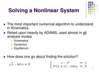
Solving a Nonlinear System. The most important numerical algorithm to understand in Kinematics Relied upon heavily by ADAMS, used almost in all analysis modes Kinematics Dynamics Equilibrium How does one go about finding the solution?. Newton-Raphson Method.

Solving a Nonlinear System
E N D
Presentation Transcript
Solving a Nonlinear System • The most important numerical algorithm to understand in Kinematics • Relied upon heavily by ADAMS, used almost in all analysis modes • Kinematics • Dynamics • Equilibrium • How does one go about finding the solution?
Newton-Raphson Method • Start by looking at the one-dimension case: • Find solution x* of the equation (root of the function): • Assumption: • The function is twice differentiable
Newton-Raphson Method • Algorithm • Start with initial guess x(0) and then compute x(1), x(2), x(3), etc. • This is called an iterative algorithm: • First you get x(1), then you improve the predicted solution to x(2), then improve more yet to x(3), etc. • Iteratively, you keep getting closer and closer to the actual solution
¢ STEP x f ( x ) f ( x ) 0 2 3 . 5838 3 . 0678 - = 1 2 3 . 0678 / 3 . 5838 1 . 1439 2 . 7109 0 . 3775 - = 2 1 . 1439 0 . 3775 / 2 . 7109 1 . 004 2 . 5451 0 . 0107 Newton-Raphson Example The exact answer is x* = 1.0
Understanding Newton’s Method • What you want to do is find the root of a function, that is, you are looking for that x that makes the function zero • The stumbling block is the nonlinear nature of the function • Newton’s idea was to linearize the nonlinear function • Then look for the root of this new linear function that hopefully approximates well the original nonlinear function • If the only thing that you have is a hammer, then make all your problems a nail
Understanding Newton’s Method(Cntd.) • You are at point q(0) and linearize using Taylor’s expansion • After linearization, you end up with linear approximation h(q) of f(q): • Find now q(1) that is the root of h, that is:
Newton-RaphsonThe Multidimensional Case • Solve for the nonlinear system • The algorithm becomes • The Jacobian is defined as
Example: Solve nonlinear system: % Use Newton method to solve the nonlinear system % x-exp(y)=0 % log(1+x)-cos(y)=0 % provide initial guess x = 1; y = 0; % start improving the guess disp('Iteration 1'); residual = [ x-exp(y) ; log(1+x)-cos(y) ]; jacobian = [1 -exp(y) ; 1/(1+x) sin(y)]; correction = jacobian\residual; x = x - correction(1) y = y - correction(2) disp('Iteration 2'); residual = [ x-exp(y) ; log(1+x)-cos(y) ]; jacobian = [1 -exp(y) ; 1/(1+x) sin(y)]; correction = jacobian\residual; x = x - correction(1) y = y - correction(2) Initial guess: x = 1 y = 0 Iteration 1 x = 1.6137 y = 0.6137 Iteration 2 x = 1.5123 y = 0.4324 Iteration 3 x = 1.5042 y = 0.4085 Iteration 4 x = 1.5040 y = 0.4081 Iteration 5 x = 1.5040 y = 0.4081
Putting things in perspective… • Newton algorithm for nonlinear systems requires: • A starting point q(0) from where the solution starts being searched for • An iterative process in which the approximation of the solution is gradually improved:
Example: Position Analysis of Mechanism • Problem 3.5.6, modeled with reduced set of generalized coordinates (see posted solution) • Iterations carried out like:
Dumb approach, which nonetheless works… % Problem 3.5.6 % Solves the nonlinear system associated with Position Analysis % Numerical solution found using Newton's method. % get a starting point, that is, an initial guess q = [0.2 ; 0.2 ; pi/4] time = 0; % start improving the guess %%%%%%%%%%%%%%%%%%%%%%%%%%%%%%% disp('Iteration 1'); dummy1 = q(1) - 0.6 + 0.25*sin(q(3)); dummy2 = q(2) - 0.25*cos(q(3)); dummy3 = q(1)*q(1) + q(2)*q(2) - (time/10+0.4)*(time/10+0.4); residual = [ dummy1 ; dummy2 ; dummy3 ]; jacobian = [1 0 0.25*cos(q(3)) ; 0 1 0.25*sin(q(3)); 2*q(1) 2*q(2) 0]; correction = jacobian\residual; q = q - correction %%%%%%%%%%%%%%%%%%%%%%%%%%%%%%% disp('Iteration 2'); dummy1 = q(1) - 0.6 + 0.25*sin(q(3)); dummy2 = q(2) - 0.25*cos(q(3)); dummy3 = q(1)*q(1) + q(2)*q(2) - (time/10+0.4)*(time/10+0.4); residual = [ dummy1 ; dummy2 ; dummy3 ]; jacobian = [1 0 0.25*cos(q(3)) ; 0 1 0.25*sin(q(3)); 2*q(1) 2*q(2) 0]; correction = jacobian\residual; q = q – correction %%%%%%%%%%%%%%%%%%%%%%%%%%%%%%% disp('Iteration 3'); dummy1 = q(1) - 0.6 + 0.25*sin(q(3)); dummy2 = q(2) - 0.25*cos(q(3)); dummy3 = q(1)*q(1) + q(2)*q(2) - (time/10+0.4)*(time/10+0.4); residual = [ dummy1 ; dummy2 ; dummy3 ]; jacobian = [1 0 0.25*cos(q(3)) ; 0 1 0.25*sin(q(3)); 2*q(1) 2*q(2) 0]; correction = jacobian\residual; q = q - correction %%%%%%%%%%%%%%%%%%%%%%%%%%%%%%% disp('Iteration 4'); dummy1 = q(1) - 0.6 + 0.25*sin(q(3)); dummy2 = q(2) - 0.25*cos(q(3)); dummy3 = q(1)*q(1) + q(2)*q(2) - (time/10+0.4)*(time/10+0.4); residual = [ dummy1 ; dummy2 ; dummy3 ]; jacobian = [1 0 0.25*cos(q(3)) ; 0 1 0.25*sin(q(3)); 2*q(1) 2*q(2) 0]; correction = jacobian\residual; q = q - correction %%%%%%%%%%%%%%%%%%%%%%%%%%%%%%% disp('Iteration 5'); dummy1 = q(1) - 0.6 + 0.25*sin(q(3)); dummy2 = q(2) - 0.25*cos(q(3)); dummy3 = q(1)*q(1) + q(2)*q(2) - (time/10+0.4)*(time/10+0.4); residual = [ dummy1 ; dummy2 ; dummy3 ]; jacobian = [1 0 0.25*cos(q(3)) ; 0 1 0.25*sin(q(3)); 2*q(1) 2*q(2) 0]; correction = jacobian\residual; q = q - correction
Example: Position Analysis of Mechanism • Output of the code shows how the position configuration at time t=0 is gradually improved Initial guess: q = 0.2000 0.2000 0.7854 Iteration 1: q = 0.4232 0.1768 0.7854 Iteration 2: q = 0.3812 0.1348 1.0228 Iteration 3: q = 0.3813 0.1216 1.0635 Iteration 4: q = 0.3813 0.1210 1.0654 Iteration 5: q = 0.3813 0.1210 1.0654 • After 4 iterations it doesn’t make sense to keep iterating, the solution is already very good
Better way to implement Position Analysis… % Problem 3.5.6 % Solves the nonlinear system associated with Position Analysis % Numerical solution found using Newton's method. % get a starting point, that is, an initial guess q = [0.2 ; 0.2 ; pi/4] time = 0; % start improving the guess for i = 1:6 crnt_iteration = strcat('Iteration ', int2str(i)); disp(crnt_iteration); dummy1 = q(1) - 0.6 + 0.25*sin(q(3)); dummy2 = q(2) - 0.25*cos(q(3)); dummy3 = q(1)*q(1) + q(2)*q(2) - (time/10+0.4)*(time/10+0.4); residual = [ dummy1 ; dummy2 ; dummy3 ]; jacobian = [1 0 0.25*cos(q(3)) ; 0 1 0.25*sin(q(3)); 2*q(1) 2*q(2) 0]; correction = jacobian\residual; q = q - correction end This way is better since you introduced an iteration loop and go through six iterations before you stop. Compared to previous solution it saves a lot of coding effort and makes it more clear and compact
Even better way to implement Position Analysis… % Problem 3.5.6 % Solves the nonlinear system associated with Position Analysis % Numerical solution found using Newton's method. % get a starting point, that is, an initial guess q = [0.2 ; 0.2 ; pi/4] time = 0; % start improving the guess normCorrection = 1.0; tolerance = 1.E-8; iterationCounter = 0; while normCorrection>tolerance, iterationCounter = iterationCounter + 1; crnt_iteration = strcat('Iteration ', int2str(iterationCounter)); disp(crnt_iteration); dummy1 = q(1) - 0.6 + 0.25*sin(q(3)); dummy2 = q(2) - 0.25*cos(q(3)); dummy3 = q(1)*q(1) + q(2)*q(2) - (time/10+0.4)*(time/10+0.4); residual = [ dummy1 ; dummy2 ; dummy3 ]; jacobian = [1 0 0.25*cos(q(3)) ; 0 1 0.25*sin(q(3)); 2*q(1) 2*q(2) 0]; correction = jacobian\residual; q = q - correction; normCorrection = norm(correction); end disp('Here is the value of q:'), q This way is even better since you keep iterating until the norm of the correction becomes very small…
function phi = getPhi(q, t) % computes the violation in constraints % Input : current position q, and current time t % Output: returns constraint violations dummy1 = q(1) - 0.6 + 0.25*sin(q(3)); dummy2 = q(2) - 0.25*cos(q(3)); dummy3 = q(1)*q(1) + q(2)*q(2) - (t/10+0.4)*(t/10+0.4); phi = [ dummy1 ; dummy2 ; dummy3 ]; % Problem 3.5.6 % Solves nonlinear system associated with Position Analysis % Numerical solution found using Newton's method. % get a starting point, that is, an initial guess q = [0.2 ; 0.2 ; pi/4] time = 0; % start improving the guess normCorrection = 1.0; tolerance = 1.E-8; iterationCounter = 1; while normCorrection>tolerance, residual = getPhi(q, time); jacobian = getJacobian(q); correction = jacobian\residual; q = q - correction; normCorrection = norm(correction); iterationCounter = iterationCounter + 1; end disp('Here is the value of q:'), q function jacobian = getJacobian(q) % computes the Jacobian of the constraints % Input : current position q % Output: Jacobian matrix J jacobian = [ 1 0 0.25*cos(q(3)) ; 0 1 0.25*sin(q(3)); 2*q(1) 2*q(2) 0 ];
Newton’s Method: Closing Remarks • Can ever things go wrong with Newton’s method? • Yes, there are at least three instances: • Most commonly, the starting point is not close to the solution that you try to find and the iterative algorithm diverges (goes to infinity) • Since a nonlinear system can have multiple solutions, the Newton algorithm finds a solution that is not the one sought (happens if you don’t choose the starting point right) • The speed of convergence of the algorithm is not good (happens if the Jacobian is close to being singular (zero determinant) at the root, not that common)
Newton’s Method: Closing Remarks • What can you do address these issues? • You cannot do anything about 3 above, but can fix 1 and 2 provided you choose your starting point carefully • Newton’s method converges very fast (quadratically) if started close enough to the solution • To help Newton’s method in Position Analysis, you can take the starting point of the algorithm at time tk to be the value of q from tk-1 (that is, the very previous configuration of the mechanism)
Position Analysis: Final Form % Driver for Position Analysis % Works for kinematic analysis of any mechanism % User needs to implement three subroutines: % provideInitialGuess % getPhi % getJacobian % general settings normCorrection = 1.0; tolerance = 1.E-8; timeStep = 0.05; timeEnd = 4; timePoints = 0:timeStep:timeEnd; results = zeros(3,length(timePoints)); crntOutputPoint = 0; % start the solution loop q = provideInitialGuess(); for time = 0:timeStep:timeEnd crntOutputPoint = crntOutputPoint + 1; while normCorrection>tolerance, residual = getPhi(q, time); jacobian = getJacobian(q); correction = jacobian\residual; q = q - correction; normCorrection = norm(correction); end results(:, crntOutputPoint) = q; normCorrection = 1; end function q_zero = provideInitialGuess() % purpose of function is to provide an initial % guess to start the Newton algorithm at % time=0 q_zero = [0.2 ; 0.2 ; pi/4]; function phi = getPhi(q, t) % computes the violation in constraints % Input : current position q, and current time t % Output: returns constraint violations dummy1 = q(1) - 0.6 + 0.25*sin(q(3)); dummy2 = q(2) - 0.25*cos(q(3)); dummy3 = q(1)*q(1) + q(2)*q(2) - (t/10+0.4)*(t/10+0.4); phi = [ dummy1 ; dummy2 ; dummy3 ]; function jacobian = getJacobian(q) % computes the Jacobian of the constraints % Input : current position q % Output: Jacobian matrix J jacobian = [ 1 0 0.25*cos(q(3)) ; 0 1 0.25*sin(q(3)); 2*q(1) 2*q(2) 0 ];