Acoustic Triangulation Device
500 likes | 733 Views
Group 13 Senior Design. Acoustic Triangulation Device. Project Description. The Acoustic Triangulation Device (ATD) is an electronic system designed to detect the location of a sonic event, specifically gunshots or explosions, and relay that location in real time to the user.

Acoustic Triangulation Device
E N D
Presentation Transcript
Group 13 Senior Design Acoustic Triangulation Device Group 13 - Ben Noble, Johnathan Sanders, Jeremy Hopfinger
Project Description • The Acoustic Triangulation Device (ATD) is an electronic system designed to detect the location of a sonic event, specifically gunshots or explosions, and relay that location in real time to the user. • Its main subsystems include but are not limited to a microphone array, GPS locator, and real time triangulation software. These systems will work together to determine the origin of any sonic event within a predetermined frequency range. • As will be shown, the philosophy of use is broad and the device will prove useful in a variety of applications. Group 13 - Ben Noble, Johnathan Sanders, Jeremy Hopfinger
Philosophy of Use • VIP Protection (Speeches etc.) • Inner city law enforcement • Military use • Civilian Property / National Park Regulation Group 13 - Ben Noble, Johnathan Sanders, Jeremy Hopfinger
Requirements and Specifications Group 13 - Ben Noble, Johnathan Sanders, Jeremy Hopfinger
Problem Solving Methods • There are many algorithms for locating the origin of wave based events. • The majority of these techniques require the event to occur within the area of a microphone array. • E.g. Mic B Mic A Source Mic C Group 13 - Ben Noble, Johnathan Sanders, Jeremy Hopfinger
Technique: Multilateration • Many military applications use a technique called Hyperbolic Multilateration. • In this technique the time difference of arrival (TDOA) of an acoustic event between two microphones limits the possibility of a source location to one half of a hyperbola. Group 13 - Ben Noble, Johnathan Sanders, Jeremy Hopfinger
Multilateration • A second and third TDOA are obtained from a second and third microphone. • These TDOAs produce respective second and third hyperbolae. • The intersection of the hyperbolae is the location of the source. • In order to have an accurate measurement for the speed of sound which we will subsequently refer to as C, we will need the temperature T. Group 13 - Ben Noble, Johnathan Sanders, Jeremy Hopfinger
Multilateration • Due to the fact that there is a constant distance differential along the hyberbolae this method can easily be derived from the distance formula. • Here A, B, and C reference microphones A, B and C respectively. Group 13 - Ben Noble, Johnathan Sanders, Jeremy Hopfinger
Multilateration • Unfortunately since we do not know the exact time the sonic event initially occurs we cannot know the time it takes the sound wave to travel to the closest microphone (in this case mic A). • We do however have the TDOA between A and all subsequent microphones, therefore we can translate the source location to A. Group 13 - Ben Noble, Johnathan Sanders, Jeremy Hopfinger
Multilateration • Also if we choose an origin for the system at microphone A then we can simplify further. • This means that the locations for microphone B and C are relative locations with respect to microphone A. • There are then two equations and two unknowns which are the x-coordinate and y-coordinate for the sound source. Group 13 - Ben Noble, Johnathan Sanders, Jeremy Hopfinger
Multilateration • This can be easily expanded to the 3 dimensional case using a 3rd dimensional hyperboloid. • All this takes is one additional mic and a third equation. Group 13 - Ben Noble, Johnathan Sanders, Jeremy Hopfinger
Problems • Accuracy improvement in Multilateration involves a technique known as Nonlinear Least-Squares Stochastic Gradient Regression. • This technique involves more microphones and is an advanced way of averaging the perceived source location from each mic. • Needless to say, this is difficult, time consuming, and increases the price of the unit due to additional equipment. • Our initial design required eight microphones for accurate results. Group 13 - Ben Noble, Johnathan Sanders, Jeremy Hopfinger
Problems • Suppose we have an acoustic event located 400 meters away from the unit oriented directly in front of mic A with microphones spaced 1 meter apart (as per specifications). • This yields the equations: where A and B are the TDOA’s. • Solving this yields B=0.00206025 seconds, A=0.00206025 seconds (intuitively both TDOA’s are the same for this configuration) Mic B 400 m Mic A Source Mic C Group 13 - Ben Noble, Johnathan Sanders, Jeremy Hopfinger
Problems • Now suppose we have an acoustic event located 405 meters away from the unit oriented directly in front of mic A. with microphones spaced 1 meter apart. • This yields the equations: where A and B are the TDOA’s. • Solving this yields B=0.00206026 seconds, A=0.00206026 seconds Mic B 405 m Mic A Source Mic C Group 13 - Ben Noble, Johnathan Sanders, Jeremy Hopfinger
Problems • Problem: A 5 meter difference in position yielded only a .00000001 second TDOA differential. That is 10 nanosecond difference. • In order to be accurate to within 5 meters we must sample nearly 100 million times a second for each of 8 microphones. • This would require a 800 MHz sample rate. • This along with the clock time for each instruction (assignment statements, conditional operators etc.) needed to process each sample, would require a very expensive processor. • A microcontoller with this processor would push the project out of budget, as would a PC sound card with 8 inputs. Group 13 - Ben Noble, Johnathan Sanders, Jeremy Hopfinger
Technique: Triangulation • For 2-dimensional triangulation we need 2 arrays of 3 microphones each, oriented in an equilateral triangle. • Each array will give us an angle which tells us the direction of the source. • Using these two directions and the known distance between the two arrays we can determine the sound source’s location. • If the microphones are close enough together and the sound source is sufficiently far away we can assume the sound wave approaches as a straight line perpendicular to the line originating from the source. Group 13 - Ben Noble, Johnathan Sanders, Jeremy Hopfinger
Triangulation • We can find the distance Δx1 using the distance formula. • C is the speed of sound and tB – tA is the difference between the time of first detection and the time of second detection. • Knowing the distance Δx and the side of the array S we can find the angle θ1 using trigonometry. Group 13 - Ben Noble, Johnathan Sanders, Jeremy Hopfinger
Triangulation • We can find the angle α1 based on its relationship with θ1 • These equations will work regardless of the orientation of the array, therefore the times tA and tB will always be the time that the first and second microphones detect a sonic event, respectively. • Based on these equations the sound source could be from either side of the line which connects the first and second microphones. The third microphone tells us that the source came from the opposite side that it is located. Group 13 - Ben Noble, Johnathan Sanders, Jeremy Hopfinger
Triangulation • The relationship between the β angles and the α angles are determined by knowing the orientation of each array with respect to the line L. • This information will be determined using a compass. • In this case: Group 13 - Ben Noble, Johnathan Sanders, Jeremy Hopfinger
Triangulation • Then using the Law of Sines we can determine the distance from the first array to the sound source. • The coordinates for the sound source are found by adding each portion of the distance (vertical and horizontal) to the coordinates of the GPS for the first array. Group 13 - Ben Noble, Johnathan Sanders, Jeremy Hopfinger
Triangulation • Combining these equations we get α for each array. • We can also combine the previous equations to find D. Group 13 - Ben Noble, Johnathan Sanders, Jeremy Hopfinger
Triangulation • Notice that there are two equations which can tell us the value of Δy1. • If these two equations are not equal then there is some amount of error in the system. • Setting the two equations equal allows us to solve for an expected angle and compare that angle with the one found in the previous equations. Group 13 - Ben Noble, Johnathan Sanders, Jeremy Hopfinger
Triangulation • The same equations apply to the 3D case except that the speed of sound is broken into two parts. • These two equations can be solved simultaneously and will give us a horizontal angle and a vertical angle. • The same method can then be used as before to determine the exact location of the sound source. Group 13 - Ben Noble, Johnathan Sanders, Jeremy Hopfinger
Solutions • Lets return to the same event located 400 meters away from the unit oriented directly in front of mic A of the first array with mics spaced 1 m apart and 10 m between arrays. • This yields the equations: where t1 and t2 are the TDOA’s. • Solving this yields t1=0.00248763 seconds, t2=0.00252485 seconds Mic B 400 m Mic A Source Mic C Group 13 - Ben Noble, Johnathan Sanders, Jeremy Hopfinger
Solutions • Now lets look at the event located 405 meters away from the unit oriented directly in front of mic A of the first array with mics spaced 1 m apart and 10 m between arrays. • This yields the equations: where t1 and t2 are the TDOA’s. • Solving this yields t1=0.00248810 seconds, t2=0.00252485 seconds. The second time being the same due to the angle not changing. Mic B 405 m Mic A Source Mic C Group 13 - Ben Noble, Johnathan Sanders, Jeremy Hopfinger
Solutions • This time a 5meter difference in position yielded only a .00000047 second TDOA differential. That is 470 nanosecond difference. • This is a significant decrease in necessary sample rate. The sample rate required for this worst case scenario which used only 6 microphones is 12MHz. • This allowed us to use a significantly cheaper microcontroller. Group 13 - Ben Noble, Johnathan Sanders, Jeremy Hopfinger
Code Sample • This short piece of code shows the pre-scale factor for an ADC. • At maximum speed an ADC loses some ability to give an accurate analogue voltage reading. • After some trial and error we determined that a pre-scale factor of 16 was a good average between accuracy and speed. Group 13 - Ben Noble, Johnathan Sanders, Jeremy Hopfinger
Signal Analysis • Wavelet Vs. Fourier Transforms • Time Domain Signal: • The Fourier transform shows the frequency spectrum of the time domain signal. • Fourier Transform: Frequency Domain Signal Group 13 - Ben Noble, Johnathan Sanders, Jeremy Hopfinger
Signal Analysis • Problem: Notice that the Fourier transform graph tells us nothing about the times at which a frequency occurs. • Example: Observe the following two signals. (Note: Both the signals contain only the frequencies 5, 10, 20, and 50 Hz) Stationary Non-Stationary Group 13 - Ben Noble, Johnathan Sanders, Jeremy Hopfinger
Signal Analysis • Problem: The Fourier transform of both functions provides the same frequency response graph. • Both signals contain the same frequencies at different times. Note that the Fourier graph cannot provide any time information at all… whatsoever. • This means Fourier analysis is useless for distinguishing between non-stationary audio signals. (Most audio signals) Group 13 - Ben Noble, Johnathan Sanders, Jeremy Hopfinger
Signal Analysis • How can we solve this problem? • One approach is the Short Time Fourier Transform (STFT). • In this method the wave to be analyzed is broken up into time segments via a window function • The window function lets us correlate different frequencies to different times and as the STFT is just a Fourier transform in two variables, we can again graph the result. Group 13 - Ben Noble, Johnathan Sanders, Jeremy Hopfinger
Signal Analysis • Notice now that for each frequency there exists a band in time, with a certain amplitude (amount of that frequency, in that time band) • Notice also that the width in frequency is small but non-zero. • This indicates that the frequency resolution is not perfect. We should have impulse responses at 5, 10, 20, and 50 Hz. • Instead there are bands around these frequencies. • This is known as frequency resolution and the wider the band, the poorer the resolution. Group 13 - Ben Noble, Johnathan Sanders, Jeremy Hopfinger
Signal Analysis • Recall, the Heisenberg uncertainty principal. • The same principal can be applied to the time and frequency information of a signal. Poor Frequency Resolution Poor Time Resolution Group 13 - Ben Noble, Johnathan Sanders, Jeremy Hopfinger
Signal Analysis • To solve the problem of resolution, we will use wavelets in our signal analysis. • Note: This is a STFT (a FT windowed in time) but windowed in frequency as well. • The window function (psi in the equation) is now a frequency/time window and is known as the mother wavelet. • Note that Psi is varied in time and scaled in frequency. Group 13 - Ben Noble, Johnathan Sanders, Jeremy Hopfinger
Signal Analysis • Examples of suitable mother wavelets: Group 13 - Ben Noble, Johnathan Sanders, Jeremy Hopfinger
Daubechies 4th Mother Wavelet Group 13 - Ben Noble, Johnathan Sanders, Jeremy Hopfinger
Signal Analysis • Gun shot comparison: • By using the wavelet transforms of prerecorded gunshots and comparing the frequency time wavelet coefficients to an event currently occurring, we can distinguish between gunshot types with a high degree of accuracy. Group 13 - Ben Noble, Johnathan Sanders, Jeremy Hopfinger
Components • Microphones • Knowles MD9745APZ-F • Omni directional • Flat frequency response • Operates at 5V • Highly Sensitive • Cheap • Very small • Came with 100x preamp Group 13 - Ben Noble, Johnathan Sanders, Jeremy Hopfinger
Components • Development Board • Arduino Mega • Microcontroller ATmega1280 • 16 Analog Inputs • 16 Mhz clock speed • 128kb Flash memory • Easy to program using C++ Group 13 - Ben Noble, Johnathan Sanders, Jeremy Hopfinger
Components • GPS • EM 408 • Extremely high sensitivity : -159dBm • 5m Positional Accuracy • Cold Start : 42s • 75mA at 3.3V • 20 gram weight • Outputs NMEA 0183 binary protocol Group 13 - Ben Noble, Johnathan Sanders, Jeremy Hopfinger
Components • Compass • HMC-6352 • 2.7 to 5.2V supply range • Simple I2C interface • 1 to 20Hz selectable update rate • 0.5 degree heading resolution • 1 degree repeatability Group 13 - Ben Noble, Johnathan Sanders, Jeremy Hopfinger
Components • Temperature Sensor • DS18B20 Digital Temperature Sensor • ± 0.5º C accuracy from -10º C to +85 º C • Converts temperature to 12-bit digital word in a max of 750ms • Operates at 3.3 V Group 13 - Ben Noble, Johnathan Sanders, Jeremy Hopfinger
Design Summary Group 13 - Ben Noble, Johnathan Sanders, Jeremy Hopfinger
Design Summary Group 13 - Ben Noble, Johnathan Sanders, Jeremy Hopfinger
Administrative Content Budget Group 13 - Ben Noble, Johnathan Sanders, Jeremy Hopfinger
Administrative Content • For the duration of the project our group worked together to accomplish all goals. • Each member however had a specific area of expertise. Work Distribution Group 13 - Ben Noble, Johnathan Sanders, Jeremy Hopfinger
Special Thanks • RobiPolikar – Rowan University The Wavelet Tutorial • Special thanks to RobiPolikar for allowing us to use pictures from his website at • http://users.rowan.edu/~polikar/WAVELETS/WTtutorial.html • Special thanks to Louis Scheiferedecker for allowing us to use several of his firearms for testing. Group 13 - Ben Noble, Johnathan Sanders, Jeremy Hopfinger