Confidence intervals
Confidence intervals. Summer program Brian Healy. Last class. Central limit theorem Hypothesis testing Null and Alternative hypotheses Test statistic p-value Conclusion. What are we doing today?. Confidence interval Comparison between confidence interval and hypothesis testing

Confidence intervals
E N D
Presentation Transcript
Confidence intervals Summer program Brian Healy
Last class • Central limit theorem • Hypothesis testing • Null and Alternative hypotheses • Test statistic • p-value • Conclusion
What are we doing today? • Confidence interval • Comparison between confidence interval and hypothesis testing • Practice problems • How to do this in R • R functions
Steps for hypothesis testing • State type of test and alpha level • State null and alternative hypotheses • Determine and calculate appropriate test statistic • Calculate p-value • Decide whether to reject or not reject the null hypothesis • NEVER accept null • Write conclusion
Example • A former student of mine collected a large amount of demographic data from school children in Afghanistan. Since this population was possibly malnourished, she was concerned that the children would have a hemoglobin level below the healthy average. The healthy average is 13 g/dL. • She asked me to run a hypothesis test comparing the hemoglobin levels in her sample population to the healthy average value. She had collected a sample of size 127 children. • Sample hemoglobin levels: • Mean = 11.7 g/dL • Standard deviation = 1.2 g/dL
Steps for hypothesis testing • We are doing a one-sample test with alpha=0.05 • Hypotheses • H0: m=13 g/dL • HA: m != 13 g/dL • p-value < 0.0001 • Reject null hypothesis • Conclusion: There is a significant difference between the average hemoglobin levels in the children in Afghanistan and the normal average hemoglobin level
Something more • Up to this point we have drawn a sample and estimated the population value with the sample mean. This was called a point estimate. • Beyond the simple point estimate, we have used the standard deviation of the sample to allow us to test hypotheses about the population mean. The only problem was that we could only answer Yes or No about the hypothesis test. • Now, we may want to know even more than the point estimate and the specific hypothesis test results so that we know an interval of plausible values for the population mean based on our sample • Confidence interval
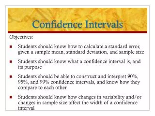
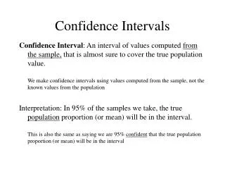
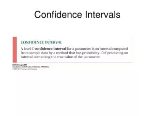
Confidence interval • Definition: a set of values that we believe are plausible estimates of population mean based on the sample we have drawn • As we discussed yesterday, when we take multiple samples, the sample mean will not be the same every time (in fact it will almost certainly be different). The confidence interval is an interval around our sample mean that allows us to have a certain amount of confidence that the true mean is covered by the interval. • We can draw conclusions about the true population mean based on our confidence interval
Example • Although the hypothesis test for our children told us that the average hemoglobin level is lower than the average level in the United States, we have learned very little about the actual health of the children. Beyond the point estimate of the population mean, my former student was interested in knowing what was the plausible range of values for the population mean hemoglobin level because she knows that her sample mean is a function of her sample. Basically, she would like to know, “How accurate was this 11.7 value?”. This would allow her to see how the children compare to other countries and decide on possibe interventions.
Construction of a confidence interval • To construct a confidence interval we need to go back to probability… • We are going to start with a standard normal. Remember that 1.96 leaves 0.025 in the upper tail in a standard normal RV. Note that we are using the population variance .
The probability statement now says something about m, but remember m is not a random variable • The resulting interval we get is, which means that we are 95% confident that this interval will cover m • We must be careful about the interpretation: • This does NOT mean “m falls within this interval 95% of the time” or “95% of the population values lie between these limits” or “there is a 95% chance that m is in the interval” because m is a specific value • This does mean “if we selected 100 random samples from the population and calculated 100 confidence intervals for m, approximately 95 of the intervals would cover m and 5 would not • A more general confidence interval is
Illustration • Let’s look at this through a simulation • www. • Note that we do not always cover the population mean exactly 95 times out of 100, but on average we will. • What can you say about the 95% and 99% confidence intervals?
Changing the width of the confidence interval • The width of the confidence interval is based on 3 factors • confidence level (z)- how confident do we want to be that the interval covers m; the higher the confidence, the wider the interval • variance (s)- how different might the samples be; the more variability, the wider the interval • sample size (n)- how many samples did we use to estimate the population mean; the larger the sample, the better the point estimate, the narrower the interval
Practice • We would like to provide a 95% confidence interval for the hemoglobin level for the children in the school. Assume we know the population variance is equal to the sample variance • For a 99% interval,
Conclusions • We are 95% confident that the true mean level of hemoglobin in school children is between 11.49 and 11.91. Beyond that, we are 99% confident that the true mean level is between 11.43 and 11.97. • We cannot say that there is a 95% chance that the true mean level of hemoglobin is between and because either the true mean is in the interval or not. • Remember that our confidence interval is subject to the same sampling variability as the hypothesis test in that sometimes just by chance our confidence interval will not cover the true population mean.
One-sided confidence interval • These are very common in everyday life (catching a bus or train), but far less common in statistical applications • These are either a lower (upper) bound because instead of being 95% confident that the mean is in an interval, we now say that we are 95% confident that the mean is above (below) a given value. To have 0.05 in the lower (upper) tail, the cut-off from the standard normal distribution is -1.645 (1.645). How could we have found this value in R?
One-sided continued • The 95% one-sided confidence interval (lower bound) is • The 95% one-sided confidence interval (upper bound) is • The interpretation of these are “we are 95% confident that m is at most (at least) the given upper bound (lower bound).
Confidence interval with the t-distribution • As we discussed yesterday, often we do not know the population standard deviation. In these cases, we need to use the sample standard deviation and the t-distribution. • The entire procedure for finding the confidence interval is the same as for the normal confidence interval, but the cut-offs are from the t-distribution. Remember the degrees of freedom for the t-distribution are the total sample size minus 1 (n-1)
Confidence intervals in R • Anytime you perform a hypothesis test in R a confidence interval is given as well • t.test(vector, [alternative=], conf.level=.95) • The confidence interval will be one-sided or two-sided based on the alternative • Remember that the default hypothesis test is that m=0, so the p-value you get may not be relevant • Practice: write a function that allows the user to input a sample vector, the population standard deviation, and the confidence level and outputs a normal two-sided confidence interval
Example • Let’s build a confidence interval for our hemoglobin using t.test • hemolevel<-read.table(“g:\\ \\hemolevel.dat”, header=T) • t.test(hemolevel) One Sample t-test data: hemolevel t = 111.4219, df = 125, p-value < 2.2e-16 alternative hypothesis: true mean is not equal to 0 95 percent confidence interval: 11.49530 11.91105 sample estimates: mean of x 11.70317 • Now, let’s build a one-sided 99% lower confidence interval • t.test(hemolevel, alternative=“greater”, conf.level=.99) t = 111.4219, df = 125, p-value < 2.2e-16 alternative hypothesis: true mean is greater than 0 99 percent confidence interval: 11.45565 Inf
Comparison of hypothesis testing and confidence interval • Let’s try a couple of hypothesis tests for our hemoglobin level • t.test(hemolevel, mu=13): our test from before • t.test(hemolevel, mu=12) • t.test(hemolevel, mu=11.9) • t.test(hemolevel, mu=11.91105) • What happens to the p-value in each of these cases? • Conclusions?
As you can see, if you would reject a specific null hypothesis (H0: m=m0), this value is not included in the confidence interval. Therefore, you can use a confidence interval to test a hypothesis just as well as you use a hypothesis test. • The reason for this relationship is because a confidence interval is the inversion of the hypothesis test, meaning that the confidence interval could have been constructed by finding all of the values of m for which the hypothesis test would fail to reject.
Possible function for normal confidence interval normalci<-function(data, stand, level){ n<-nrow(data) xbar<-mean(data) zalpha<- -qnorm((1-level)/2) ll<-xbar-zalpha*(stand/sqrt(n)) ul<- xbar+zalpha*(stand/sqrt(n)) list(lowerlim=ll,upperlim=ul) } > normalci(hemolevel,2,0.95) $lowerlim hemoglobin 11.35396 $upperlim hemoglobin 12.05239


