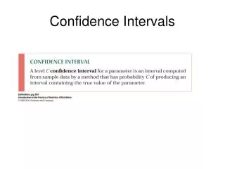
Confidence intervals
Confidence intervals. Kristin Tolksdorf (based on previous EPIET material) 18 th EPIET /EUPHEM Introductory course 01 . 10 .201 2. Inferential statistics. Uses patterns in the sample data to draw inferences about the population represented, accounting for randomness .

Confidence intervals
E N D
Presentation Transcript
Confidence intervals Kristin Tolksdorf(based on previous EPIET material) 18thEPIET/EUPHEM Introductory course 01.10.2012
Inferential statistics • Uses patterns in the sample data to draw inferences about the population represented, accounting for randomness. • Two basic approaches: • Hypothesis testing • Estimation
Criticism on significance testing “Epidemiological application need more than a decision as to whether chance alone could have produced association.” (Rothman et al. 2008) →Estimation of an effect measure(e.g. RR, OR) rather than significance testing. →Estimation of a mean →Estimation of a proportion
Why estimation? Norovirus outbreak on a Greek island: “The risk of illness was higher among people who ate raw seafood (RR=21.5).” How confident can we be in the result? What is the precision of our point estimate?
The epidemiologist needs measurements rather than probabilities 2 is a test of association OR, RR are measures of association on a continuous scale infinite number of possible values The best estimate = point estimate Range of “most plausible” values, given the sample data Confidence interval precision of the point estimate
Confidence interval (CI) Range of values, on the basis of the sample data, in which the population value (or true value) may lie. • Frequently used formulation: „If the data collection and analysis could be replicated many times, the CI should include the true value of the measure95% of the time.”
Confidenceinterval (CI) a = 5% 1 - α α/2 α/2 s Lower limit upper limit of 95% CI of 95% CI 95% CI = x – 1.96 SEuptox + 1.96 SE Indicates the amount of random error in the estimate Can becalculatedforany „teststatistic“, e.g.: means, proportions,ORs, RRs
CI terminology Point estimate Confidence interval RR = 1.45 (0.99 – 2.13) Lower confidence limit Upper confidence limit
Width of confidence interval depends on … • amount of variability in the data • size of the sample • level of confidence (usually 90%, 95%, 99%) A common way to use CI regarding OR/RR is : If 1.0 is included in CI non significant If 1.0 is not included in CI significant
A B Large RR RR = 1 Looking at the CI Study A, large sample, precise results, narrow CI – SIGNIFICANT Study B, small size, large CI - NON SIGNIFICANT Study A, effect close to NO EFFECT Study B, no information about absence of large effect
1 RR 20 studies with different results... More studies are better or worse? clinical or biological significance ?
Norovirus on a Greek island • How confident can we be in the result? • Relative risk = 21.5 (point estimate) • 95% CI for the relative risk: (8.9 - 51.8) The probability that the CI from 8.9to 51.8 includes the true relative risk is 95%.
Norovirus on a Greek island “The risk of illness was higher among people who ate raw seafood (RR=21.5, 95% CI 8.9 to 51.8).”
Example: Chlordiazopoxide use and congenital heart disease (n=1 644) OR = (4 x 1250) / (4 x 386) = 3.2 p = 0.080 ; 95% CI=0.6 - 17.5 From Rothman K
3.2 p=0.080 0.6 – 17.5
Example: Chlordiazopoxide use and congenital heart disease – large study (n=17 151) OR = (240 x 8800) / (211 x 7900) = 1.3 p = 0.013 ; 95% CI=1.1 -1.5
Precision and strength of association Strength Precision
Confidence interval provides more information than p value • Magnitude of the effect (strength of association) • Direction of the effect (RR > or < 1) • Precision of the point estimate of the effect (variability) p value can not provide them !
What we have to evaluate the study • 2Test of association, depends on sample size • p valueProbability that equal (or more extreme) results can be observed by chance alone • OR, RRDirection & strength of association if > 1 risk factor if < 1 protective factor (independently from sample size) • CI Magnitude and precision of effect
Comments on p-values and CIs • Presence of significance does not prove clinical or biological relevance of an effect. • A lack of significance is not necessarily a lack of an effect: “Absence of evidence is not evidence of absence”.
Comments on p-values and CIs • A huge effect in a small sample or a small effect in a large sample can result in identical pvalues. • A statistical test will always give a significant result if the sample is big enough. • p values and CIs do not provide any information on the possibility that the observed association is due to bias or confounding.
2 and Relative Risk Cases Non-cases Total 2 = 1.3 E 9 51 60 p = 0.13 NE 5 55 60 RR = 1.8 Total 14 106 120 95% CI [ 0.6 - 4.9 ] Cases Non-cases Total 2 = 12 E 90 510 600 p = 0.0002 NE 50 550 600 RR = 1.8 Total 140 1060 1200 95% CI [ 1.3-2.5 ]
Common source outbreak suspected Exposure Cases Non-cases AR% Yes 15 20 42.8% No 50 200 20.0% Total 65 220 2 = 9.1 p = 0.002 RR = 2.1 95%CI= 1.4 - 3.4 23% REMEMBER: These values do not provide any information on the possibility that the observed association is due to a bias or confounding.
The ultimative (eye) test • Hypothesis testing: X²-Test • Question: Is the proportion of facilitators wearing glasses equal to the proportion of fellows wearing glasses? • Estimation of quantities: Proportion • What is the proportion of fellows/facilitators wearing glasses?
The ultimative (eye) test Glasses among fellows : Yes 11 No 27 Total 38 Glasses among facilitators : Yes 6 No 8 Total 14 Proportion = 11/38 = 0.29 SE = 0.074 95%CI = 0.14 - 0.44 Proportion = 6/14 = 0.43 SE = 0.132 95%CI = 0.17 - 0.69
Recommendations • Always look at the raw data (2x2-table). How many cases can be explained by the exposure? • Interpret with caution associations that achieve statistical significance. • Double caution if this statistical significance is not expected. • Use confidence intervals to describe your results.
Suggested reading • KJ Rothman, S Greenland, TL Lash, Modern Epidemiology, Lippincott Williams & Wilkins, Philadelphia, PA, 2008 • SN Goodman, R Royall, Evidence and Scientific Research, AJPH 78, 1568, 1988 • SN Goodman, Toward Evidence-Based Medical Statistics. 1: The P Value Fallacy, Ann Intern Med. 130, 995, 1999 • C Poole, Low P-Values or Narrow Confidence Intervals: Which are more Durable? Epidemiology 12, 291, 2001
Previous lecturers • Alain Moren • Paolo D’Ancona • Lisa King • Preben Aavitsland • Doris Radun • Manuel Dehnert • ÁgnesHajdu

