Download

1 / 12
120 likes | 247 Views
This lecture covers Error-Correcting Learning and the Least Mean Square (LMS) algorithm, fundamental concepts in supervised learning. It explains the process of feedback from the environment, the significance of minimizing square error, and how LMS adjusts weights based on error. Cases of linear and nonlinear activations are discussed, along with practical examples and MATLAB applications. The lecture aims to deepen understanding of error correction techniques and their role in optimizing learning algorithms.

E N D
Lecture 7.Learning (IV):Error correcting Learning and LMS Algorithm
Outline • Error Correcting Learning • LMS algorithm • Nonlinear activation • Batch mode Least Square Learning (C) 2001-2003 by Yu Hen Hu
xM(n) wM d(n): feedback from environment u(n) y(n) w1 x1(n) w0 Supervised Learning with a Single Neuron Input: x(n) = [1 x1(n) … xM(n)]T Parameter: w(n) = [w0(n) w1(n) … wM(n)]T Output: y(n) = f[u(n)] = f[wT(n)xT(n)] Feedback from environment: d(n), desired output. (C) 2001-2003 by Yu Hen Hu
Error-Correction Learning • Error @ time n = desired value – actual value e(n) = d(n) – y(n) • Goal: modify w(n) to minimized square error E(n) = e2(n) • This leads to a steepest descent learning formulation: w(n+1) = w(n) – ' wE(n) where wE(n) = [E(n)/w0(n) … E(n)/wM(n)]T = 2 e(n) [y(n)/w0(n) … y(n)/wM(n)]T is the gradient of E(n) w.r.t. w(n). ’ is a learning rate constant. (C) 2001-2003 by Yu Hen Hu
Case 1. Linear Activation: LMS Learning If f(u) = u, then y(n) = u(n) = wT(n)x(n) Hence wE(n) =2 e(n) [y(n)/w0(n) … y(n)/wM(n)]T = 2 e(n) [1 x1(n) … xM(n)]T = 2 e(n) x(n) Note e(n) is a scalar, and x(n) is a M+1 by 1 vector. Let = 2’, we have the least mean square (LMS) learning formula as a special case of error-correcting learning: w(n+1) = w(n) + h e(n)•x(n) Observation The amount of corrections made to w(n), w(n+1)w(n) is proportional to the magnitude of the error e(n) and along the direction of the input vector x(n). (C) 2001-2003 by Yu Hen Hu
Example Let y(n) = w0(n) •1+ w1(n) x1(n) + w2(n) x2(n). Assume the inputs are: Assume w0(1) = w1(1) = w2(1) = 0, and = 0.01. e(1) = d(1) – y(1) = 1 – [0•1 + 0•0.5 + 0•0.8] = 1 w0(2) = w0(1) + e(1)•1 = 0 + 0.01•1•1 = 0.01 w1(2) = w1(1) + e(1) x1(1) = 0 + 0.01•1•0.5 = 0.005 w2(2) = w2(1) + e(1) x2(1) = 0 + 0.01•1•0.8 = 0.008 (C) 2001-2003 by Yu Hen Hu
Results Matlab source file: Learner.m (C) 2001-2003 by Yu Hen Hu
Case 2. Non-linear Activation In general, Observation: The additional terms is f’ [u(n)]. When this term becomes small, learning will NOT take place. Otherwise, the update formula is similar to LMS. (C) 2001-2003 by Yu Hen Hu
LMS and Least Square Estimate Assume that the parameters w remain unchanged for n = 1 to N (> M). Then, e2(n) = d2(n) 2d(n)wTx(n) + wTx(n)xT(n)w. Define an expected error (Mean square error) Denote Then where R: correlation matrix, : cross correlation vector. (C) 2001-2003 by Yu Hen Hu
Least Square Solution • Solve wE = 0, for W, we have wLS = R1 • When {x(n)} is a wide-sense stationary random process, the LMS solution w(n) converges in probability to the least square solution wLS. LMSdemo.m (C) 2001-2003 by Yu Hen Hu
LMS Demonstration (C) 2001-2003 by Yu Hen Hu
LMS output comparison (C) 2001-2003 by Yu Hen Hu