Quantitative Genetics
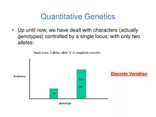
Quantitative Genetics. พีระพงษ์ แพงไพรี. ความแตกต่างของสองลักษณะ. Qualitative traits. Quantitative traits. ควบคุมด้วยยีนมากคู่ สิ่งแวดล้อมมีผลมาก ต้องชั่ง ตวง วัด. ควบคุมด้วยยีนน้อยคู่ สิ่งแวดล้อมมีผลน้อย แยกหมวดหมู่ได้. P = G + E + ( GxE ). P = Phenotype G = Genetic or Genotype


Quantitative Genetics
E N D
Presentation Transcript
Quantitative Genetics พีระพงษ์ แพงไพรี
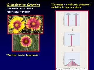
ความแตกต่างของสองลักษณะความแตกต่างของสองลักษณะ Qualitative traits Quantitative traits ควบคุมด้วยยีนมากคู่ สิ่งแวดล้อมมีผลมาก ต้องชั่ง ตวง วัด • ควบคุมด้วยยีนน้อยคู่ • สิ่งแวดล้อมมีผลน้อย • แยกหมวดหมู่ได้
P = G + E + (GxE) P = Phenotype G = Genetic or Genotype E = Environment GxE = Genetic - Environment interaction
P = G + E additive gene G = A + D + I epistasis effect permanent environment dominant effect E = Ep +Et temporary environment P = A + D + I + Ep + Et
P = A + D + I + Ep + Et 2P= 2A+2D+2I+2Ep+2Et additive gene
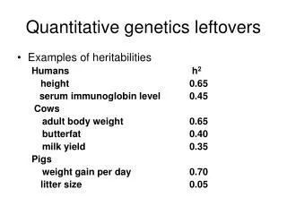
2P= 2A+2D+2I+2Ep+2Et 2A = อัตราพันธุกรรม (heritability, h2) 2P หมายถึง สัดส่วนความแปรปรวนเนื่องจากพันธุกรรม ต่อ ความแปรปรวนทั้งหมด
ประเภทของอัตราพันธุกรรมประเภทของอัตราพันธุกรรม 1 2G = board sense heritability, h2B 2P 2 2A = narrow sense heritability, h2N 2P
ระดับของอัตราพันธุกรรมระดับของอัตราพันธุกรรม สูง = > 0.35 คุณภาพ ผลผลิต ปานกลาง= 0.20 - 0.35 ต่ำ = < 0.20 การสืบพันธุ์, การอยู่รอด
แนวทางการใช้ประโยชน์ สูง ปานกลาง ต่ำ no heterosis no yes selection program cross breed management program
การคำนวณหา h2 • sib analysis • half-sib analysis • full-sib analysis • regression between parent and offspring
half-sib analysis 2sire sire 1 sire 2 sire 3 2offspring/sire = 2W Yij = + sirei + offspring/sirej/i
half-sib analysis 2sire sire 1 sire 2 sire 3 2offspring/sire = 2W
2total = 2sire +2W = 2P COVhalf sib = ¼ 2A = 2sire 42sire = 2A
ANOVA Yij = + sirei + offspring/sirej/i k = จำนวนลูกต่อพ่อ 2W = MSW 2sire = (MSS – MSW) k
ANOVA Yij = + sirei + offspring/sirej/i 20 18,000 900 10,800 9 1,200 29 28,800 2W = 900 k = 3 2sire = (1,200 – 900) = 100 3
full-sib analysis 2Sire 2Dam 2W Dam 1 Dam 2 sire 1 sire 2 Yij = + sirei + dam/sirej/i+ offspring/dam/sirei/j/k
full-sib analysis 2Sire 2Dam 2W Dam 1 Dam 2 sire 1 sire 2
2P = 2Sire+2Dam+2W COVfull sib = ½2A+¼2D = 2Sire+2Dam 2(2sire+2Dam)= 2A+ ½2D COVhalf sib = ¼2A = 2Sire 42sire = 2A
42sire = 2A 42Dam = 2A+2D 2(2sire+2Dam)= 2A+ ½2D COVfull sib-half sib= ¼2A+¼2D = 2Dam 42Dam = 2A+2D
42sire = 2A 42Dam = 2A+2D 2(2sire+2Dam)= 2A+ ½2D 42sire = 2A 2A h2 = _____ 2P 2P 42Dam = 2A+2D 2P 2(2sire+2Dam)= 2A+ ½2D 2P
ANOVA Yij = + sirei + dam/sirej/i+ offspring/dam/sirei/j/k 2sire = (MSS – MSD) k2 2Dam = (MSD – MSW) k1 2W = MSW k1 = จำนวนลูกต่อแม่ k2 = จำนวนลูกต่อพ่อ
ANOVA Yij = + sirei + dam/sirej/i+ offspring/dam/sirei/j/k 490 10 49 657 1,980 33 9 60 73 3,127 79 2W = 33 2Sire = 3 2sire = (73 – 49) 8 2Dam = (49 – 33) 4 2Dam = 4 k1 = 4 k2 = 8
2Sire = 3 2Dam = 4 2W = 33 42sire = 2A 2P 2A 42Dam = 2A+2D h2 = _____ 2P 2P 2(2sire+2Dam)= 2A+ ½2D 2P
regression between parent and offspring ½ 2A = b COV(แม่,ลูก) b = __________ 2b = 2A V(แม่)
COV(แม่,ลูก) = 100 b = ______________ V(แม่) = 1000 b = 0.1 h2 = 2b = 2(0.1) = 0.2
2G 2EP
2P= 2A+2D+2I+2Ep+2Et 2G+2Ep = อัตราซ้ำ (repeatability, t) 2P หมายถึง สัดส่วนความแปรปรวนเนื่องจากพันธุกรรม และสิ่งแวดล้อมถาวร ต่อ ความแปรปรวนทั้งหมด
2W 2e 2W = 2G + 2EP 2e = 2ET 2W t = __________ 2W+2e
ANOVA k = จำนวนข้อมูลต่อตัว 2e = MSe 2W = (MSW– MSe) k
ANOVA 20 9,000 450 19,800 9 2,200 29 28,800 2e = 450 k = 3 2W = (2,200 – 450) = 583 3
0 h2 1 0 t 1
genetic correlation (rG) สหสัมพันธ์ทางพันธุกรรม (rG) • pleiotropy • genetic linkage -1 rG +1
+ FCR 0 ADG
FCR - 0 ADG
XY r= ____________ 2X 2Y
half-sib analysis ADG 2SADG 2S 2SFCR FCR SADGFCR 2WADG ADG sire 1 sire 2 sire 3 2W 2WFCR FCR
ANOVA ADG 2SADG FCR 2SFCR
ANCOVA SADGFCR SADGFCR r= _________________ 2SADG 2SFCR
ANOVA ADG 2SADG = 75 FCR 2SFCR = 165
ANCOVA 2SADG = 75 2SFCR = 165 SADGFCR= 80