Download
1 / 16
270 likes | 860 Views
Continuum Representations of the Solvent. pp. 502 - 512 (Old Edition) Eva Zurek. Surface Types. van der Waals Surface: is constructed from the overlapping vdW spheres of the atoms

E N D
Continuum Representations of the Solvent pp. 502 - 512 (Old Edition) Eva Zurek
Surface Types • van der Waals Surface: is constructed from the overlapping vdW spheres of the atoms • Molecular Surface: is traced out by the inward-facing part of the probe sphere as it rolls on the vdW surface of the molecule. Usually defined using a water molecule (sphere, radius 1.4 A) as the probe. • Contact surface: consists of regions where the probe is in contact with the vdW surface. • Re-entrant surface: regions occur where there are crevices too narrow for the probe molecule to penetrate. • The Accessible Surface: is the surface traced by the center of the probe molecule.
Solute Solvent Solvent Solute Dielectric continuum; e How to Model the Solvent? • Solvent molecules are directly involved in the reaction; the solvent molecules are tightly bound to the solute explicit solvation. • The solvent provides a ‘bulk medium’; the dielectric properties of the solvent are of primary importance continuum solvation models.
The Free Energy of Solvation • DGsol the free energy change to transfer a molecule from vacuum to solvent. • DGsol = DGelec + DGvdw + DGcav (+ DGhb) An explicit hydrogen bonding term. Electrostatic component. Free energy required to form the solute cavity. Is due to the entropic penalty due to the reorganization of the solvent molecules around the solute and the work done in creating the cavity. Van der Waals interaction between solute and solvent.
e a q The Born Model • Born, 1920: the electrostatic component of the free energy of solvation for placing a charge in a spherical solvent cavity. • The solvation energy is equal to the work done to transfer the ion from vacuum to the medium. This is the difference in work to charge the ion in the two environments. • Ionic radii from crystal structures is used. • Only relevant for species with a formal charge.
The Generalized Born (GB) Equation, Classical • Consider a system of N particles with radii ai and charges qi in a medium of relative permittivity e.
Implementations of GB • The GB equation has been incorporated into MM calculations by Still et al. where: • When i = j this expression returns the Born equation; for two charges close together the expression returns the Onsager result (ie. a dipole where rij ai, aj); for two charges very far apart (rij ai, aj)) it is close to sum of Coulomb and Born expressions. • Advantage: the expression can be differentiated analytically; therefore fast geometry optimizations!
Gruesome Detail You Really Don’t Want to Know So I Won’t Talk About It • A rather complex procedure is used to determine the Born radii in Still’s implementation. In short, The Born radius of an atom corresponds to the radius that would return the electrostatic energy of the system according to the Born equation if all of the other molecules in the system were uncharged. • In Cramer and Truhlar’s QM approach the radius of the atom is a function of the charge on the atom.
e a The Onsager Model • Onsager, 1936: considers a polarizable dipole with polarizability a at the center of a sphere. • The solute dipole induces a reaction field in the surrounding medium which in turn induces an electric field in the cavity (reaction field)which interacts with the dipole.
Classical Onsager • If the species is charged an appropriate Born term must be added. • Other Models: A point dipole at the center of a sphere (Bell), A quadrupole at the center of a sphere (Abraham), multipole expansion to represent the solute, ellipsoidal and molecular cavities.
Quantum Onsager Self-Consistent Reaction Field • The reaction field is a first-order perturbation of the Hamiltonian. Correction factor corresponding to the work done in creating the charge distribution of the solute within the cavity in the medium
The Cavity in the Onsager Model • Spherical and ellipsoidal cavities may be used • Advantage: analytical expressions for the first and second derivatives may be obtained • Disadvantage: this is rarely true! • How does one define the radius value? • For a spherical molecule the molecular volume, Vm can be found: • Estimate by the largest interatomic distance • Use an electron density contour Radii • Often the radius obtained from these procedures is increased to account for the fact that a solvent particle can not approach right up to the molecule
The Polarizable Continuum Method (PCM) • The van der Waals radii of the atoms are used to determine the cavity surface. • The surface is divided into a number of small surface elements with area DS. • If Ei is the electric field gradient at pt i due to the solute then an initial charge, qi is assigned to each element via: • The potential due to the point charges, fs(r) is found, giving a new electric field gradient. The charges are modified until they converge. • The solute Hamiltonian is modified: • After each SCF new values of qi and fs(r) are computed.
The PCM Approach • Problems: • Since the continuous charge distribution is discretized when the electrostatic potential due to the charges on the surface elements is calculated for a given element i, the charge on i must be excluded otherwise the charges would diverge • The contribution of the charge on this surface element is found separately using the Gauss theorem • Due to the fact that the wavefunction extends outside the cavity the sum of the charges on the surface is not equal and opposite to the charge of the solute outlying charge error • The charge distribution may be scaled so that this is true Work done in creating the charge distribution within the cavity in the dielectric medium.
The Conductor-like Screening Model (COSMO) • The dielectic is replaced with a conductor. To pass from a conductor to the dielectric an empirical factor is introduced. Thus, • For the classical case the energy of the system is, where C is the Coulomb matrix, Bim represents the interaction between two unit charges placed at the position of the solute charge Qi and the apparent charge qm,and Amn represents the interaction between two unit charges at qm and qn. • These eq’s may also be derived from the boundary condition of vanishing potential on the surface of a conductor (f = 0).
Applications • The effect of solvent upon energetics and equilibria ie, the tautomeric equilibria of 2-pyridone: • The calculated free energy differences were calculated as being -0.64 kcal/mol, 0.36 kcal/mol and 2.32 kcal/mol in gas phase, cyclohexane (non-polar) and acetonitrile (polar) in good comparison with experiment. • The medium was found to have a greater influence on the keto rather than the enol form since the keto tautomer is more polar.