Quicksort

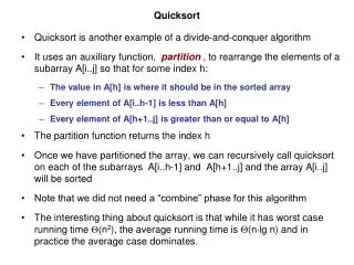
1. Quicksort • Quicksort is another example of a divide-and-conquer algorithm • It uses an auxiliary function, partition , to rearrange the elements of a subarray A[i..j] so that for some index h: • The value in A[h] is where it should be in the sorted array • Every element of A[i..h-1] is less than A[h] • Every element of A[h+1..j] is greater than or equal to A[h] • Thepartition function returns the index h • Once we have partitioned the array, we can recursively call quicksort on each of the subarrays A[i..h-1] and A[h+1..j] and the array A[i..j] will be sorted • Note that we did not need a “combine” phase for this algorithm • The interesting thing about quicksort is that while it has worst case running time (n2), the average running time is (nlg n) and in practice the average case dominates.

2. Quicksort • The partition algorithm uses index variables h and k and sets a pivot value x = A[i] • The idea is that at the beginning of each iteration of the key for-loop we have: • For all r satisfying i+1 ≤ r ≤ h , A[r] < x • For all r satisfying h+1 ≤ r ≤ k-1, A[r]  x • nothing definite is known about the values in A[k..j] • The algorithm moves k one index to the right each time through the for-loop until it reaches j • The index h is advanced only when k encounters a value less than the pivot value • When this happens, h is moved forward one position and the value in that position (which we know is  x) is swapped for the value at position k (which we know is < x) • At the end, we switch A[i] with the value in position h (which we know is less than x), and return h.

3.  x Partition Note that if A[i+1] < A[i], in the first pass through the loop, we increment h to be i+1, which is also the value of k; so the swap doesn’t do anything! Partition(A,i,j) • x = A[i] • h = i • for k= i+1 to j • doif A[k] < x • then h = h+1 • swap(A[h], A[k]) • swap( A[i], A[h] ) • return h Loop invariants: 1. i+1  r  h  A[r] < x 2. h+1  r  k-1  A[r]  x i h k j x unrestricted < x

4. < x  x ? Example: Partition

5. < x  x ? Example: Partition

6. < x  x ? Example: Partition

7. < x  x ? Example: Partition

8. < x  x ? Example: Partition

9. < x  x ? Example: Partition

10. < x  x ? Example: Partition

11. < x  x ? Example: Partition

12. < x  x ? Example: Partition

13. < x  x ? Example: Partition

14. < x  x ? Example: Partition

15. Quicksort Quicksort(A,i,j) • if i < j • then h = Partition(A,i,j) • Quicksort(A,i,h-1) • Quicksort(A,h+1,j)

16. Performance • It should be clear that partition runs in (n) time, where n is the number of elements in the subarray A[i..j. • The worst case for quicksort is when the partition function provides subarrays of size n-1 and 0 whenever it is called • In this case, the running time function is given by the recurrence T(n) = T(n-1) + T(0) + (n) = T(n-1) + (n) • This recurrence gives T(n) being (n2) • The best case is when partition gives two equal size partitions, one of size n/2 and the other of size n/2-1 • This gives the recurrence T(n) = 2T(n/2) + (n), yielding a running time which is (nlg n). • Interestingly enough, the best running time is realized whenever all the partitions are split with any constant proportionality (1/10 to 9/10, etc) not just 1/2 to 1/2.

17. Randomized Quicksort • Often in an average-case analysis of an algorithm (such as quicksort), we assume that every possible array permutation is equally likely • That is, we assume a uniform random distribution • In practice, we may not be able to rely on this assumption • One way around this is to build randomness into our algorithm • We could randomly permute the given array before applying the algorithm • The following code segment will do that: for i = 1 to n-1 swap( A[i], A[random(i,n)] )

18. Randomized Quicksort • The approach we take for randomized quicksort is called randomized sampling: • We randomly select a value in the array and swap it with the value in A[i], which now becomes our pivot value Randomized-Partition(A,i,j) • r= random(i,j) • swap( A[r], A[i] ) • return Partition(A,i,j) Randomized-Quicksort(A,i,j) if i < j then h = Randomized-Partition(A,i,j) Randomized-Quicksort(A,i,h-1) Randomized-Quicksort(A,h+1,j)

19. Analysis of Quicksort • Worst Case prove by induction that T(n) is (n2) T(n) = max0≤q ≤n-1( T(q) + T(n-q-1)) + (n) Show that T(n) ≤ cn2 for some constant c T(n) ≤ max0≤q ≤n-1( cq2 + c(n-q-1)2) + (n) = max0≤q ≤n-1 c( q2 + (n-q-1)2) + (n) The function q2 + (n-q-1)2 achieves its maximum at the endpoints of the interval 0 ≤ q ≤ n-1. (Simple calculus) Thus the maximum is less equal to (n-1)2 and thus T(n) is O(n2) We previously gave an example where Quicksort ran in time n2 and therefore the worst-case running time of Quicksort is also (n2)

20. Harmonic Numbers • The nth harmonic number is the sum of the first n integer reciprocals Hn = 1 + 1/2 + 1/3 +  + 1/n • We would like to give an asymptotic bound for the nth harmonic number. • One convenient way is to use the integral from calculus • Integrals can be used to give bounds for arbitrary increasing functions

21. The sum of the areas of the rectangles is The area under y = f(x) from x = m-1 to n is Therefore: Using Integrals to Bound Summations

22. The sum of the areas of the rectangles is The area under y = f(x) from x = m to n+1 is Therefore: Using Integrals to Bound Summations

23. Using Integrals to Bound Summations Thus we have If we apply this to the function f(k) = 1/k, we have It then follows that Thus we have shown that is (lg n)

24. Expected Running Time of Randomized Quicksort • The running time for Quicksort is dominated by the time spent in the Partition algorithm • In Quicksort, first Partition is called • This rearranges the elements of the array into three subarrays: • left, containing values less than the pivot value; • middle, consisting of the pivot value only; and • right, containing the values greater than or equal to the pivot value • Then Quicksort is used recursively to sort the left and right subarrays • Note that the pivot value is never again involved in a call to Quicksort • Thus there are at most n calls to Partition, where n is the number of elements in the subarray • Each call to Partition takes O(1) time plus a constant times the number of iterations of the for-loop.

25. Expected Running Time of Randomized Quicksort • Each call to Partition takes O(1) time plus a constant times the number of iterations of the for-loop. • Each iteration of the for-loop does the comparison “A[k]  x?” exactly once for each value of k. • Thus if we can count the total number of times line 4 is, we can bound the total time spent in the for-loop during the entire execution of Quicksort • This count can be used to give an upper bound on the running time of Quicksort • Partition(A,i,j) • x = A[i] • h = i • for k= i+1 to j • doifA[k] < x • then h = h+1 • swap(A[h], A[k]) • swap( A[i], A[h] ) • return h

26. Expected Running Time of Randomized Quicksort • LemmaLet X be the number of times the comparison in line 4 of Partition is executed over the entire execution of Quicksort. Then the running time of Quicksort is O(n + X). • Recall that we are considering Randomized-Quicksort, which we claim to be O(n lg n)

27. Expected Running Time of Randomized Quicksort • In general, the number of times the comparison is executed depends on the way in which the array is partitioned at each stage • Recall that we are considering Randomized-Quicksort, which we claim to be O(n lg n) • At some point in the analysis, we will use the randomization to accomplish our task • We will not consider counting comparisons in each individual call to Partition • Rather, we will look at the total number of comparisons throughout the execution of Quicksort • So we need to know when two elements will be compared and when they will not be compared.

28. Expected Running Time of Randomized Quicksort • We need to know when two elements will be compared and when they will not be compared. • First note that any given pair of elements will be compared at most one time • Why? Elements are only compared to a pivot element and once that particular call to Partition ends, the pivot value is never again involved in a comparison • Let z1, z2, . . . , zn be the elements of the array in nondecreasing order. • Define the set Zij = { zi, zi+1, . . . , zj } • Let Xij = I{ zi is compared to zj over the entire execution of Quicksort}| • Then the total number of comparisons is |S| denotes the cardinality of set S

29. Expected Running Time of Randomized Quicksort • Then the total number of comparisons is • Taking expectations of both sides: • So now we need to compute Pr{ zi is compared to zj } • Recall that we assume that each pivot is chosen independently and randomly

30. Expected Running Time of Randomized Quicksort • We need to compute Pr{ zi is compared to zj } • Assumption: each pivot is chosen independently and randomly • Once a pivot x is chosen it is compared with every element in the subarray. • If zi  x  zj, we know that zi will not be compared to zj after the current call to Partition terminates. • Why? Because they are in separate partitions and thus will not be in the same subarray for subsequent calls to Quicksort (and hence to Partition • If zi is chosen as a pivot before any other element in Zij, then it will be compared to every other element in that set except itself. • The same holds true for zj. • Thus zi and zj will be compared if and only if the first element in Zij to be chosen as a pivot is either zi or zj.

31. Expected Running Time of Randomized Quicksort • zi and zj will be compared if and only if the first element in Zij to be chosen as a pivot is either zi or zj. • Pivot values are chosen independently and randomly, • Thus each element of Zij has the same probability for being the first element of Zij to be chosen as the pivot. • Since there are j-i+1 elements in Zij , that probability is • Thus

32. Expected Running Time of Randomized Quicksort • We use a change of variables k = j-i below:

33. Selection • The median of an array of elements is the “middle” value in the array • One may want to know the kth smallest element in the array • The median would be the n/2th smallest element • This problem is called the selection problem: given an array A and a valid index k, find the kth smallest element in A. • One obvious approach is to sort and access A[k] • But the running time is then (nlogn) and we can do better

34. Selection • All the practical selection algorithms are based on the partition algorithm • If we run partition and x happens to be placed at index k, we are done. • If it is placed at an index > k, we can restrict our search to the left part of the partition, otherwise at the right part. • This leads to a recursive approach similar to quicksort • Just as in the case of quicksort, the worst case running time is (n2) • And as before, we go to randomized partition to get a better running time

35. Randomized Select • Randomized-Select(A, i, j, k) //returns the kth smallest element in A[i..j]// precondition: 1  k  j-i+1 if (i = j) thenreturn A[i] h = Randomized-Partition(A,i,j) p = h - i + 1 // A[h] is the pth smallest element in A[i..j] if p = k thenreturn A[h] else if (k < p) // kth smallest element comes before pth smallest element = A[h] thenreturn Randomized-Select (A,i,h-1,k) else return Randomized-Select (A,h+1,j,k-p)

36. Running Time of Randomized-Select • Theorem The expected running time for Randomized-Select is (n) Proof Let cn be the expected time for input A[1], …, A[n] If n >1, the instruction p = randomized_partition(A,i,j) takes time n-1. Thus cn is (n) If p  k, random_select is called recursively on an array of size p-1 or on an array of size n-p. Thus the expected time for the recursive call is at most max { cp-1, cn-p } and this holds even if p = k Since all indices are equally likely, We now prove by induction that if c1  1, then cn≤ 4c1n for n > 1.

37. Running Time Continued • Claim: if c1  1, then cn≤ 4c1n for n > 1; proof by induction on n The basis step n = 1 is obvious For the inductive step, assume cp ≤ 4c1p for all p < n. Then

38. Quicksort Homework • Page 252: #2, #7 • Page 267: # 5