Quicksort
Explore Quicksort performance analysis, design, pseudocode, and correctness proofs from a noted computer science professor's lecture slides. Learn about worst-case and average-case execution times, partitioning strategies, and empirical studies. Compare Quicksort with other sorting algorithms.


Quicksort
E N D
Presentation Transcript
Quicksort Ack: Several slides from Prof. Jim Anderson’s COMP 202 notes. Comp 122, Spring 2004
Performance • A triumph of analysis by C.A.R. Hoare • Worst-case execution time – (n2). • Average-case execution time – (n lg n). • How do the above compare with the complexities of other sorting algorithms? • Empirical and analytical studies show that quicksort can be expected to be twice as fast as its competitors. Comp 122
Design • Follows the divide-and-conquer paradigm. • Divide:Partition (separate) the array A[p..r] into two (possibly empty) subarrays A[p..q–1] and A[q+1..r]. • Each element in A[p..q–1] A[q]. • A[q] each element in A[q+1..r]. • Index q is computed as part of the partitioning procedure. • Conquer: Sort the two subarrays by recursive calls to quicksort. • Combine: The subarrays are sorted in place – no work is needed to combine them. • How do the divide and combine steps of quicksort compare with those of merge sort? Comp 122
Pseudocode Partition(A, p, r) x, i := A[r], p – 1; for j := p to r – 1 do if A[j] x then i := i + 1; A[i] A[j] fi od; A[i + 1] A[r]; return i + 1 Quicksort(A, p, r) if p < r then q := Partition(A, p, r); Quicksort(A, p, q – 1); Quicksort(A, q + 1, r) fi A[p..r] 5 A[p..q – 1] A[q+1..r] Partition 5 5 5 Comp 122
Example p r initially: 2 5 8 3 9 4 1 7 10 6note: pivot (x) = 6 i j next iteration:2 5 8 3 9 4 1 7 10 6 i j next iteration:25 8 3 9 4 1 7 10 6 i j next iteration:2 58 3 9 4 1 7 10 6 i j next iteration:2 538 9 4 1 7 10 6 i j Partition(A, p, r) x, i := A[r], p – 1; for j := p to r – 1 do if A[j] x then i := i + 1; A[i] A[j] fi od; A[i + 1] A[r]; return i + 1 Comp 122
Example (Continued) next iteration:2 538 9 4 1 7 10 6 i j next iteration:2 5389 4 1 7 10 6 i j next iteration:2 534 98 1 7 10 6 i j next iteration:2 534189 7 10 6 i j next iteration:2 5341897 10 6 i j next iteration:2 5341897106 i j after final swap:2 5341697108 i j Partition(A, p, r) x, i := A[r], p – 1; for j := p to r – 1 do if A[j] x then i := i + 1; A[i] A[j] fi od; A[i + 1] A[r]; return i + 1 Comp 122
Partitioning • Select the last element A[r] in the subarray A[p..r] as the pivot– the element around which to partition. • As the procedure executes, the array is partitioned into four (possibly empty) regions. • A[p..i] — All entries in this region are pivot. • A[i+1..j – 1] — All entries in this region are > pivot. • A[r] = pivot. • A[j..r – 1] — Not known how they compare to pivot. • The above hold before each iteration of the for loop, and constitute a loop invariant. (4 is not part of the LI.) Comp 122
Correctness of Partition • Use loop invariant. • Initialization: • Before first iteration • A[p..i] and A[i+1..j – 1] are empty – Conds. 1 and 2 are satisfied (trivially). • r is the index of the pivot – Cond. 3 is satisfied. • Maintenance: • Case 1:A[j] > x • Increment j only. • LI is maintained. Partition(A, p, r) x, i := A[r], p – 1; for j := p to r – 1 do if A[j] x then i := i + 1; A[i] A[j] fi od; A[i + 1] A[r]; return i + 1 Comp 122
Correctness of Partition i r j p >x x > x x j i r p x > x x Case 1: Comp 122
Correctness of Partition i r j p x x > x x i j r p x > x x • A[r] is unaltered. • Condition 3 is maintained. • Case 2:A[j] x • Increment i • Swap A[i] and A[j] • Condition 1 is maintained. • Increment j • Condition 2 is maintained. Comp 122
Correctness of Partition • Termination: • When the loop terminates, j = r, so all elements in A are partitioned into one of the three cases: • A[p..i] pivot • A[i+1..j – 1] > pivot • A[r] = pivot • The last two lines swap A[i+1] and A[r]. • Pivot moves from the end of the array to between the two subarrays. • Thus, procedure partition correctly performs the divide step. Comp 122
Complexity of Partition • PartitionTime(n) is given by the number of iterations in the for loop. • (n) : n = r – p + 1. Partition(A, p, r) x, i := A[r], p – 1; for j := p to r – 1 do if A[j] x then i := i + 1; A[i] A[j] fi od; A[i + 1] A[r]; return i + 1 Comp 122
Algorithm Performance Running time of quicksort depends on whether the partitioning is balanced or not. • Worst-Case Partitioning (Unbalanced Partitions): • Occurs when every call to partition results in the most unbalanced partition. • Partition is most unbalanced when • Subproblem 1 is of size n – 1, and subproblem 2 is of size 0 or vice versa. • pivot every element in A[p..r – 1] or pivot< every element in A[p..r – 1]. • Every call to partition is most unbalanced when • Array A[1..n] is sorted or reverse sorted! Comp 122
Worst-case Partition Analysis Recursion tree for worst-case partition Running time for worst-case partitions at each recursive level: T(n) = T(n – 1) + T(0) + PartitionTime(n) = T(n – 1) + (n) = k=1 to n(k) = (k=1 to nk ) = (n2) n n – 1 n – 2 n n – 3 2 1 Comp 122
Best-case Partitioning • Size of each subproblem n/2. • One of the subproblems is of size n/2 • The other is of size n/2 1. • Recurrence for running time • T(n) 2T(n/2) + PartitionTime(n) = 2T(n/2) + (n) • T(n) = (n lg n) Comp 122
Recursion Tree for Best-case Partition cn cn/2 cn/2 cn/4 cn/4 cn/4 cn/4 c c c c c c cn cn lg n cn cn Total : O(n lg n) Comp 122
Recurrences – II Comp 122, Spring 2004
Recurrence Relations • Equation or an inequality that characterizes a function by its values on smaller inputs. • Solution Methods (Chapter 4) • Substitution Method. • Recursion-tree Method. • Master Method. • Recurrence relations arise when we analyze the running time of iterative or recursive algorithms. • Ex: Divide and Conquer. T(n) = (1)if n c T(n) = a T(n/b) + D(n) + C(n)otherwise Comp 122
Technicalities • We can (almost always) ignore floors and ceilings. • Exact vs. Asymptotic functions. • In algorithm analysis, both the recurrence and its solution are expressed using asymptotic notation. • Ex:Recurrence with exact function T(n) = 1 if n = 1 T(n) = 2T(n/2) + n if n > 1 Solution:T(n) = n lgn + n • Recurrence with asymptotics (BEWARE!) T(n) = (1) if n = 1 T(n) = 2T(n/2) + (n) if n > 1 Solution:T(n) = (n lgn) • “With asymptotics” means we are being sloppy about the exact base case and non-recursive time – still convert to exact, though! Comp 122
Substitution Method • Guess the form of the solution, then use mathematical induction to show it correct. • Substitute guessed answer for the function when the inductive hypothesis is applied to smaller values – hence, the name. • Works well when the solution is easy to guess. • No general way to guess the correct solution. Comp 122
Example – Exact Function Recurrence: T(n) = 1 if n = 1 T(n) = 2T(n/2) + n if n > 1 • Guess:T(n) = n lgn + n. • Induction: • Basis: n = 1 n lgn + n = 1 = T(n). • Hypothesis:T(k) = k lgk + k for all k < n. • Inductive Step: T(n) = 2 T(n/2) + n • = 2 ((n/2)lg(n/2) + (n/2)) + n • = n (lg(n/2)) + 2n • = n lgn – n + 2n • = n lgn + n Comp 122
Example – With Asymptotics To Solve: T(n) = 3T(n/3) + n • Guess: T(n) = O(n lg n) • Need to prove: T(n) cn lg n, for some c > 0. • Hypothesis: T(k) ck lg k, for all k < n. • Calculate:T(n) 3c n/3lgn/3 + n c n lg(n/3) + n = c n lg n – c n lg3 + n = c n lg n – n (c lg3–1) c n lg n (The last step istrue for c 1 / lg3.) Comp 122
Example – With Asymptotics To Solve: T(n) = 3T(n/3) + n • To show T(n) = (n lg n), must show both upper and lower bounds, i.e., T(n) = O(n lg n) ANDT(n) = (n lg n) • (Can you find the mistake in this derivation?) • Show: T(n) = (n lg n) • Calculate:T(n) 3c n/3lgn/3 + n c n lg(n/3) + n = c n lg n – c n lg3 + n = c n lg n – n (c lg3–1) c n lg n (The last step istrue for c 1 / lg3.) Comp 122
Example – With Asymptotics If T(n) = 3T(n/3) + O (n), as opposed to T(n) = 3T(n/3) + n, then rewrite T(n)3T(n/3) + cn, c> 0. • To show T(n) = O(n lg n), use second constant d, different from c. • Calculate:T(n) 3d n/3lgn/3 +c n d n lg(n/3) + cn = d n lg n – d n lg3 + cn = d n lg n – n (d lg3–c) d n lg n (The last step istrue for d c / lg3.) It is OK for d to depend on c. Comp 122
Making a Good Guess • If a recurrence is similar to one seen before, then guess a similar solution. • T(n) = 3T(n/3 + 5) + n (Similar toT(n) = 3T(n/3) + n) • When n is large, the difference between n/3 and (n/3 + 5) is insignificant. • Hence, can guess O(n lg n). • Method 2: Prove loose upper and lower bounds on the recurrence and then reduce the range of uncertainty. • E.g., start with T(n) = (n) &T(n) = O(n2). • Then lower the upper bound and raise the lower bound. Comp 122
Subtleties • When the math doesn’t quite work out in the induction, strengthen the guess by subtracting a lower-order term. Example: • Initial guess: T(n)= O(n)for T(n) = 3T(n/3)+ 4 • Results in:T(n) 3c n/3 + 4= c n + 4 • Strengthen the guess to: T(n) c n – b, where b 0. • What does it mean to strengthen? • Though counterintuitive, it works.Why? T(n) 3(c n/3 – b)+4 c n –3b + 4= c n – b –(2b – 4) Therefore, T(n) c n – b, if2b –4 0orif b 2. (Don’t forget to check the base case: here c>b+1.) Comp 122
Changing Variables • Use algebraic manipulation to turn an unknown recurrence into one similar to what you have seen before. • Example: T(n) = 2T(n1/2) + lg n • Renamem = lg nand we have T(2m) = 2T(2m/2) + m • SetS(m) = T(2m)and we have S(m) = 2S(m/2) + m S(m) = O(m lg m) • Changing back from S(m)to T(n), we have T(n) = T(2m) = S(m) = O(m lg m) = O(lg n lglg n) Comp 122
Avoiding Pitfalls • Be careful not to misuse asymptotic notation. For example: • We can falsely prove T(n) = O(n)by guessingT(n) cn for T(n) = 2T(n/2) + n T(n) 2c n/2 + n c n + n = O(n) Wrong! • We are supposed to prove that T(n) c n for all n>N, according to the definition of O(n). • Remember:prove the exact form of inductive hypothesis. Comp 122
Exercises • Solution of T(n) = T(n/2) + nisO(n) • Solution of T(n) = 2T(n/2+ 17) + nisO(n lg n) • Solve T(n) = 2T(n/2) + 1 • Solve T(n) = 2T(n1/2) + 1by making a change of variables. Don’t worry about whether values are integral. Comp 122