Download
1 / 34
340 likes | 516 Views
Chapter 6: The Standard Deviation as a Ruler and the Normal Model. AP Statistics. Shifting and Rescaling Data.

E N D
Chapter 6: The Standard Deviation as a Ruler and the Normal Model AP Statistics
Shifting and Rescaling Data Suppose your class was given a test . The mean score was 85%, the median was 80%, the standard deviation was 5% and the IQR was 7%. What if I made a mistake on the test and need to add 3 points to everyone’s grade? What would happen to those summary statistics? What if, instead, I decided to multiply everyone’s grade by 1.5? Then what would happen to those summary statistics?
Shifting and Rescaling Data • Adding (or subtracting) a constant to every data value adds (or subtracts) the same constant to measures of position (mean, median, percentiles, min, max) , but will leave measures of spread (range, IQR, standard deviation) unchanged. • This represents a “shift” of the data • The shape of the distribution will remain the same.
Shifting and Rescaling Data • Multiplying (or dividing) all the data values by any constant, all measures of position (mean, median, percentiles, min, max) and all measures of spread (range, IQR, standard deviation) are multiplied (or divided) by that same constant.
The Standard Deviation as a Ruler John recently scored a 113 on Test A. The scores on the test are distributed with a mean of 100 and a standard deviation of 10. Mary took a different test, Test B, and scored 263. The scores on her test are distributed with a mean of 250 and a standard deviation of 25. Which student did relatively better on his particular test? • John did better on his test • Mary did better on her test • They both performed equally well • It is impossible to tell since they did not take the same test • It is impossible to tell since the number of students taking the test is unknown.
The Standard Deviation as a Ruler • We need to have a level playing field—we need a way to make the numbers mean the same thing. • We do that by using a z-score • A z-score measures how many standard deviations a point is from the mean • NO UNITS for a z-score
The Standard Deviation as a Ruler • Standardizing data into z-scores does not change the shape of the data. • Standardizing data into z-scores does change the center by making the mean 0. • Standardizing data into z-scores does change the spread by making the standard deviation 1 • Positive z-score –data point above mean • Negative z-score—data point below mean
Examples • The SATs have a distribution that has a mean of 1500 and a standard deviation of 250. Suppose you score a 1850. How many standard deviations away from the mean is your score? • Suppose your friend took the ACT, which scores are distributed with a mean of 20.8 and a standard deviation of 4.8. What score would your friend need to get in order to have done as well as you did on the SATs?
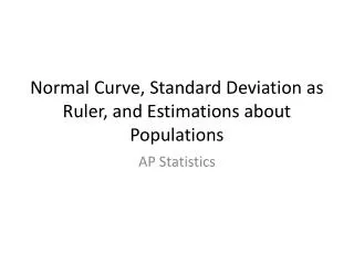
Normal Curve • When we take a sample and get real discrete data, we display it as a histogram. • This histogram also displays a good estimation of the population parameter and the shape of the true distribution. • For example, if we take a sample of 1000 people and their IQ, the sample will have a mean of 100, a standard deviation of 15, and will be normally distributed. SO WILL THE POPULATION (mostly)
Normal curve • Here is a histogram of IQ scores. The y-axis scale is in hundreds. • This sample can also be used to model the entire population.
Normal curve • We could then model the IQ scores of all adults with the density curve to the right. • This is called a standard normal model • The highest point in the graph represents the mean.
Normal Curve • The standard normal curve is a model—a model of reality –not reality itself • Therefore, the mean and standard deviation of the model are not summary statistics. They are values we use to help us specify the model. • Therefore, when we create a model for real world data we always define it by:
Standard Normal Curve • Typically, we standardize the data first (convert into z-scores)—therefore creating the standard normal curve model:
Nearly Normal Condition • When we use the normal model, we are assuming that the data is normal (symmetric). • Therefore, before you use a normal model to help in your analysis, you need to check to make sure the data is basically normal—remember, real world data is not perfectly normal • Use: Nearly Normal Condition: The shape of the data’s distribution is unimodal and symmetric
Nearly Normal Condition Two ways to check the Nearly Normal Condition • Make a histogram • Make a Normal Probability plot If the distribution of the data is roughly Normal, the plot is roughly a diagonal straight line.
Normal Probability Plot Normal Not Normal
Normal Probability Plot—calculator • We are plotting the data along the y-axis in this example
The 68-95-99.7 Rule • One of the main goals of statistics is to find out how extreme certain values are. For example, is an IQ of 110 extremely high? What about 125? • The way we do this is by determining how likely it is to find a value that far from the mean • We can find them precisely (soon) or we can find them by using the 68-95-99.7 Rule
Example The verbal section of the SAT test is approximately normally distributed with a mean of 500 and a standard deviation of 100. Approximately what percent of students will score between 400 and 600 on the verbal part of the exam? GO THROUGH COMPLETE ANSWER!!!! See pg 110 for example
Example The verbal section of the SAT test is approximately normally distributed with a mean of 500 and a standard deviation of 100. Approximately what percent of students will score above 700?
Example The verbal section of the SAT test is approximately normally distributed with a mean of 500 and a standard deviation of 100. Approximately what percent of students will score between 350 and 620? This cannot be done by using 68-95-99.7 Rule Need to use the properties of normal curve and technology
Example The verbal section of the SAT test is approximately normally distributed with a mean of 500 and a standard deviation of 100. Approximately what percent of students will score between 350 and 620?
What do you need to show? • Check Nearly Normal Condition • Draw normal curve model with proper notation (use parameter notation) • Find values you are looking for in model and shade in appropriate region • Convert to z-score • Find the area in the shaded region: • Interpret you results in context
Example The results of a placement test for an exclusive private school is normal, with a mean of 56 and a standard deviation of 12. Approximately what percent of students who take the test will score below a 40?
Example (need to find cutoff) The verbal section of the SAT test is approximately normally distributed with a mean of 500 and a standard deviation of 100. What is the lowest score someone could receive to be in the top 10% of all scores?
Example (need to find cutoff) The verbal section of the SAT test is approximately normally distributed with a mean of 500 and a standard deviation of 100. What is the lowest score someone could receive to be in the top 10% of all scores?
Example WORK The verbal section of the SAT test is approximately normally distributed with a mean of 500 and a standard deviation of 100. What is the range of the middle 50% of data?