Two-way fixed effects
Two-way fixed effects. Balanced panels i=1,2,3….N groups t=1,2,3….T observations/group Easiest to think of data as varying across states/time Write model as single observation Y it = α + X it β + u i + v t + ε it X it is (1 x k) vector. Three-part error structure

Two-way fixed effects
E N D
Presentation Transcript
Two-way fixed effects • Balanced panels • i=1,2,3….N groups • t=1,2,3….T observations/group • Easiest to think of data as varying across states/time • Write model as single observation • Yit=α + Xitβ + ui + vt +εit • Xit is (1 x k) vector
Three-part error structure • ui – group fixed-effects. Control for permanent differences between groups • vt – time fixed effects. Impacts common to all groups but vary by year • εit -- idiosyncratic error
Capture state and year effects with sets of dummy variables • di = 1 if obs from panel i (N dummies) • wt =1 if obs from time period t (T-1 dum.) • Sort data by group, year • 1st t obs from group 1 • 2nd t obs from group 2, etc
Drop constant since we have complete set of group effects • Matrix notation • Y = Xβ + Dα + Wλ + ε • D (NT x N) matrix of group dummies • W(NT x T-1) Matrix of time dummies
D looks like the matrix from one-way fixed-effects model (check your notes) • D = In it • In is N x N • it is T x 1 • D is therefore NT x N
W is tricky • 1st obs period 1, group 1 • 2nd obs period 2, group 2 • Same for all blocks i • Only t-1 dummies, but t obs • Let Wt be partitioned matrix [ It-1 / 0t-1’] • Wt is (T x (T-1)) • 1st T-1 rows are a It-1 • Final row 0t-1’ is a vector of 0’s
Wt is repeated for all N blocks of data • W = in Wt • in is (n x1), Wt is (T x (T-1)) • W is NT x (T-1)
Y = Xβ + Dα + Wλ + ε • D = In it • W = in Wt • Let H =[D | W] = [In it | in Wt] • Let Γ = [α / λ] [( N + T – 1) x 1] vector • Y = Xβ + H Γ + ε
By partitioned inverses (b is est of β) • b=[X’MX]-1[X’MY] • Mh = Int – H(H’H)-1H’ • Can show that
Mh= • Int - In(1/t)itit’ - (1/n)inin’ It + (1/nt)intint’ • Int - In(1/t)itit’ creates within panel deviations in means • Int - (1/n)inin’ It creates within year deviations in means • (1/nt)intint’ adds back sample mean
Sample within panel means of y are 0 • Sample within year means of y are 0 • Therefore, need to add back the sample mean to return the mean of the transformed y=0
Yit = β0 + X1itβ1 + … Xkitβk + ui + vt + εit • Y*it = Yit - ¥i - ¥t - ¥ • ¥i = (1/t)ΣtYit • ¥t = (1/n)ΣiYit • ¥ = [1/(nt)] ΣtΣiYit • X*1it ….. X*kit defined the same way
Estimate the model • Y*it = X*1itβ1 + … X*kitβk + εit • DOF in model are NT – K – N – (T-1)
Caution • In balanced panel, two-way fixed-effects equivalent to subtracting • Within group means • Within time means • Adding sample mean • Only true in balanced panels • If unbalanced, need to do the following
Can subtract off means on one dimension (i or t) • But need to add the dummies for the other dimension
Difference in difference models • Maybe the most popular identification strategy in applied work today • Attempts to mimic random assignment with treatment and “comparison” sample • Application of two-way fixed effects model
Problem set up • Cross-sectional and time series data • One group is ‘treated’ with intervention • Have pre-post data for group receiving intervention • Can examine time-series changes but, unsure how much of the change is due to secular changes
Y True effect = Yt2-Yt1 Estimated effect = Yb-Ya Yt1 Ya Yb Yt2 ti t1 t2 time
Intervention occurs at time period t1 • True effect of law • Ya – Yb • Only have data at t1 and t2 • If using time series, estimate Yt1 – Yt2 • Solution?
Difference in difference models • Basic two-way fixed effects model • Cross section and time fixed effects • Use time series of untreated group to establish what would have occurred in the absence of the intervention • Key concept: can control for the fact that the intervention is more likely in some types of states
Three different presentations • Tabular • Graphical • Regression equation
Y Treatment effect= (Yt2-Yt1) – (Yc2-Yc1) Yc1 Yt1 Yc2 Yt2 control treatment t1 t2 time
Key Assumption • Control group identifies the time path of outcomes that would have happened in the absence of the treatment • In this example, Y falls by Yc2-Yc1 even without the intervention • Note that underlying ‘levels’ of outcomes are not important (return to this in the regression equation)
Y Yc1 Treatment effect= (Yt2-Yt1) – (Yc2-Yc1) Yc2 Yt1 control Treatment Effect Yt2 treatment t1 t2 time
In contrast, what is key is that the time trends in the absence of the intervention are the same in both groups • If the intervention occurs in an area with a different trend, will under/over state the treatment effect • In this example, suppose intervention occurs in area with faster falling Y
Y Estimated treatment Yc1 Yt1 Yc2 control True treatment effect Yt2 True Treatment Effect treatment t1 t2 time
Basic Econometric Model • Data varies by • state (i) • time (t) • Outcome is Yit • Only two periods • Intervention will occur in a group of observations (e.g. states, firms, etc.)
Three key variables • Tit =1 if obs i belongs in the state that will eventually be treated • Ait =1 in the periods when treatment occurs • TitAit -- interaction term, treatment states after the intervention • Yit = β0 + β1Tit + β2Ait + β3TitAit + εit
More general model • Data varies by • state (i) • time (t) • Outcome is Yit • Many periods • Intervention will occur in a group of states but at a variety of times
ui is a state effect • vt is a complete set of year (time) effects • Analysis of covariance model • Yit = β0 + β3 TitAit + ui + vt + εit
What is nice about the model • Suppose interventions are not random but systematic • Occur in states with higher or lower average Y • Occur in time periods with different Y’s • This is captured by the inclusion of the state/time effects – allows covariance between • ui and TitAit • vt and TitAit
Group effects • Capture differences across groups that are constant over time • Year effects • Capture differences over time that are common to all groups
Meyer et al. • Workers’ compensation • State run insurance program • Compensate workers for medical expenses and lost work due to on the job accident • Premiums • Paid by firms • Function of previous claims and wages paid • Benefits -- % of income w/ cap
Typical benefits schedule • Min( pY,C) • P=percent replacement • Y = earnings • C = cap • e.g., 65% of earnings up to $400/month
Concern: • Moral hazard. Benefits will discourage return to work • Empirical question: duration/benefits gradient • Previous estimates • Regress duration (y) on replaced wages (x) • Problem: • given progressive nature of benefits, replaced wages reveal a lot about the workers • Replacement rates higher in higher wage states
Yi = Xiβ + αRi + εi • Y (duration) • R (replacement rate) • Expect α > 0 • Expect Cov(Ri, εi) • Higher wage workers have lower R and higher duration (understate) • Higher wage states have longer duration and longer R (overstate)
Solution • Quasi experiment in KY and MI • Increased the earnings cap • Increased benefit for high-wage workers • (Treatment) • Did nothing to those already below original cap (comparison) • Compare change in duration of spell before and after change for these two groups
Model • Yit = duration of spell on WC • Ait = period after benefits hike • Hit = high earnings group (Income>E3) • Yit = β0 + β1Hit + β2Ait + β3AitHit + β4Xit’ + εit • Diff-in-diff estimate is β3
Questions to ask? • What parameter is identified by the quasi-experiment? Is this an economically meaningful parameter? • What assumptions must be true in order for the model to provide and unbiased estimate of β3? • Do the authors provide any evidence supporting these assumptions?
Almond et al. • Babies born w/ low birth weight(< 2500 grams) are more prone to • Die early in life • Have health problems later in life • Educational difficulties • generated from cross-sectional regressions • 6% of babies in US are low weight • Highest rate in the developed world
Let Yit be outcome for baby t from mother I • e.g., mortality • Yit = α + bwitβ + Xiγ + αi + εit • bw is birth weight (grams) • Xi observed characteristics of moms • αi unobserved characteristics of moms
Terms • Neonatal mortality, dies in first 28 days • Infant mortality, died in first year
Many observed factors that might explain health (Y) of an infant • Prenatal care, substance abuse, smoking, weight gain (of lack of it) • Some unobserved as well • Quality of diet, exercise, generic predisposition • αi not included in model
Cross sectional model is of the form • Yit = α + bwitβ + Xiγ + uit • where uit =αi + εit • Cov(bwit,uit) < 0 • Same factors that lead to poor health lead to a marker of poor health (birth weight)
Solution: Twins • Possess same mother, same environmental characterisitics • Yi1 = α + bwi1β + Xiγ + αi + εi1 • Yi2 = α + bwi2β + Xiγ + αi + εi2 • ΔY = Yi2-Yi1 = (bwi2-bwi1) β + (εi2- εi1)


