Two-Way ANOVA
Two-Way ANOVA. Two-way Analysis of Variance. Two-way ANOVA is applied to a situation in which you have two independent nominal-level variables and one interval or better dependent variable

Two-Way ANOVA
E N D
Presentation Transcript
Two-way Analysis of Variance • Two-way ANOVA is applied to a situation in which you have two independent nominal-level variables and one interval or better dependent variable • Each of the independent variables may have any number of levels or conditions (e.g., Treatment 1, Treatment 2, Treatment 3…… No Treatment) • In a two-way ANOVA you will obtain 3 F ratios • One of these will tell you if your first independent variable has a significant main effect on the DV • A second will tell you if your second independent variable has a significant main effect on the DV • The third will tell you if the interaction of the two independent variables has a significant effect on the DV, that is, if the impact of one IV depends on the level of the other
The Three Effects in a Two-Way ANOVA • Let’s consider an example: What is the impact of gender, ethnicity, and their interaction on annual income? • One of these will tell you if your first independent variable has a significant main effect on the DV • What is the main effect of gender on income, regardless of (across all levels of) ethnicity? • A second will tell you if your second independent variable has a significant main effect on the DV • What is the main effect of ethnicity on income, regardless of (across all levels of) gender • The third will tell you if the interaction of the two independent variables has a significant effect on the DV • What is the combined effect of gender and ethnicity on income that could not be detected by considering the two IVs separately? (e.g., what is the interaction of gender and ethnicity with respect to income; is the effect of gender different for different categories of ethnicity?
The Null Hypotheses in a Two-Way ANOVA • The null hypotheses in a two-way ANOVA are these: • The population means for the DV are equal across levels of the first factor • The population means for the DV are equal across levels of the second factor • The effects of the first and second factors on the DV are independent of one another
An Interaction Effect in Two-Way Analysis of Variance What is the impact of gender and ethnicity on annual salary, and how do they interact? In this example, there may not be much of a main effect either for gender or ethicnity, but there may be an interaction effect: for example, are females who are Hispanic paid more than males who are Hispanic, while females who are African-American are paid less than males who are African-American?
Some Conventions to Know • For convenience purposes, one factor or IV is usually called the “column” variable and the other the “row” variable • When describing your design in the opening statement of a Method section you will refer to it as a 2 X 2 design, or a 3 X 3 design, where the first number refers to the number of levels of the row variable and the second number refers to the number of levels of the column variable. When there are more than two factors involved, in a multiple factor ANOVA, you will see 4 X 2 X 4, which means that there are three factors in the design, the first with four, the second with two, and the third with four levels of the factor. The order is usually arbitrary
More Conventions to Know • An independent variable is called a factor, and its separate impact on the DV is called a main effect • The term between effect or between-groups effect in ANOVA language refers to the differences in the DV between or among levels of a factor and is the same thing as the variable’s main effect (e.g., differences in the DV between men and women, or between African Americans and Hispanics) • The term within effect or within-groups effect in ANOVA language refers to the differences in the DV within a level of the factor (e.g., differences among the individuals within the “female” category or the “African-American” category
Various Estimates in Two-Way ANOVA • Estimates for the main effects of the two independent variables • The “between estimate,” or between mean square for the row variable (for example, ethnicity) is based on the deviation of each row mean of the DV (mean for Hispanic, mean for African-American) from the overall or grand mean of the DV • Similarly, the “between estimate,” or between mean square for the column variable, gender, is based on the deviation of each column mean of the DV (mean for females, mean for males) from the overall or grand mean of the DV • Each of these estimates is calculated as if the other factor did not exist
Estimates in Anova • The estimate or mean square for the interaction effect of gender and ethnicity is based on the deviation of the cell means (mean on the DV from each of these combinations: Hispanic/female; Hispanic/male; African-American/female; African-American/male) from the grand mean, after differences due to the two factors (gender, ethnicity) acting independently and the error variance (individual variability within the cells) have been accounted for or “removed”
Within Estimate and F Ratio, Two-Way ANOVA • The estimate or mean square for the within-cell variance is based on the deviation of each score on the DV from the mean of its own cell. It is usually called the error term (error being whatever you can’t explain by factors and their interaction) • Whenever the independent variables are regarded as “fixed,” (levels are not randomly sampled) the F ratios for the two factors (gender, ethnicity) and their interaction are calculated by dividing the appropriate main effect or interaction effect estimate by the within estimate • The degrees of freedom (DF) associated with each of the F ratios (Factor 1 main effect, Factor 2 main effect, their interaction) are k-1 and j-1, respectively, for each of the main effects, where k and j are the number of levels of the respective factors; df for the interaction term is (k-1)(j-1); and the df for the error term is N-jk
Two-Way ANOVA, Example of F tests • Test of the impact of sex and race on socioeconomic status: • Significant main effect for race (see red dots) • No significant main effect for sex (see green dots) • No significant interaction of race and sex (see blue dots) Factors (main effects and interaction effect)
Two-Way ANOVA, Example of F Tests, Cont’d According to the Levene test the group variances are significantly different so we will use the Tamhane post hoc test instead of Sheffe to see which group means are significantly different. We will only do a test on the factors for which the main effect was significant According to the Tamhane test the means for blacks and whites in Socioeconomic status were significantly different, but neither group was significantly different from “other”
Plots of Main Effects and Interaction Effect Plot of interaction effect: Note that the lines for males (red) and females (green) are very similar although there is a tiny bit of an interaction effect in the Other category where women are actually higher than men
Two-Way ANOVA, SPSS example • Suppose you hypothesized that the amount of time a person spent on the Internet each week was influenced by two factors, their educational level and their marital status. (This will be a 3 X 2 design with three levels of education (high school only, some post-high school, and college degree or more), and two levels of marital status (married/with partner or not married/with partner). • Your first hypothesis was that the more educated people are, the more time they will spend on the net. • Your second hypothesis was that the amount of time people spend on the net is likely to be influenced by their marital status, such that persons without partners are more likely to spend time on the net than those who are married/have a partner. • Your third hypothesis is that education level and marital status will interact, but you don’t predict the nature of the interaction • Main effects may be “interpreted” in a straightforward way (treated as independent of one another and interpreted individually) only if there is no significant interaction present; otherwise the interpretation of the main effects must take the interaction into account
SPSS Output, Two-Way ANOVA:Tests of Main Effects of Marital Status and Educational Level and Their Interaction on Time Spent on the Net • Tests of Hypotheses: • There is no significant main effect for education level (F(2, 58) = 1.685, p = .194, partial eta squared = .055) • There is no significant main effect for marital status (F (1, 58) = .441, p = .509, partial eta squared = .008) • There is a significant interaction effect of marital status and education level (F (2, 58) = 3.586, p = .034, partial eta squared = .110)
Deconstructing the Interaction Effect • Since there were no significant main effects for either educational level or marital status, we won’t do any post-hoc (Sheffe, Tamhane) tests of the differences between pairs of levels of the factors (for example, between high school and some post-high school) • However, we do want to examine the interaction effect since it was significant. Note how the direction of the difference in time spent on the net reverses itself for married vs. not married as a function of level of education, particularly high school vs. some post-high school
Plots of Main Effects (non-significant) of Marital Status and Education Level Generally, although the results are not significant, it would appear that unmarried or non-partnered people spend more time on the net, and net use peaks with the post-high school group and declines for college grads
Plots of Interaction Effect of Education Level and Marital Status on Time Spent on the Net Education Level is plotted along the horizontal axis and hours spent on the net is plotted along the vertical axis. The red and green lines show how marital status interacts with education level. If marital status had the same effect on time spent on the net across all levels of education, the lines would be more or less parallel. In an interaction effect, they cross or diverge from parallel in some way. Here we note that the general trend for single people to spend more time on the net is very strong for the post-high school group but is reversed for high school grads and college grads, where married people spend more time What do you think might explain this?
Step-by-step Two-Way ANOVA in SPSS • First, download the socialsurveysmall.sav data file • We are going to test the hypotheses that • Sex of respondent has a significant main effect on hours per day spent watching TV • Home ownership has a significant main effect on hours per day spent watching TV • Sex of respondent and home ownership have a significant interaction effect on hours per day spent watching TV • Go to Analyze/General Linear Model/ Univariate • Move the variables Respondent’s Sex and OwnsOwnHome into the Fixed Factor window • Move the Hours per Day Watching TV variable into the Dependent Variables window • Click on Model, select Full Factorial, and Continue • Ignore the Contrasts Button for now
Step-by-Step Two-Way ANOVA in SPSS • Next, we are going click on the Plots button to select the plots we want. • First we get plots for the main effects • Move the Sex factor into the Horizonal Axis window and click the Add button • Move the Homeown factor into the Horizontal Axis window and click the Add button • Next we will get plots for the interaction effect • Move the Sex factor into the Horizontal Axis window and the Homeown factor into the Separate Lines window and click the Add button • Move the Homeown factor into the Horizontal Axis window and the Sex factor into the Separate Lines window and click the Add button • Click Continue
Step-by-step Two-Way ANOVA in SPSS • We will skip the post-hoc tests button this time because our variables only have two levels each and the post-hoc tests are only performed when there are more than two levels. Otherwise you do the post hoc tests just as you did for one-way ANOVA by moving the factors you want to test into the Post Hoc Tests box and selecting Sheffe and Tamhane tests • Click on Options and move all of the Factors (overall, Sex, Homeown, and Sex*Homeown) into the Display Means for box • Check Compare Main Effects, Descriptives, Estimates of Effect Size, Observed Power, and Homogeneity Tests, and set the confidence interval to 95% • Click Continue and then OK • Compare your output to the next several slides
Your SPSS Output for Two-Way ANOVA 1. Sex of respondent has a significant main effect on hours per day spent watching TV 2. Home ownership has a significant main effect on hours per day spent watching TV 3. Sex of respondent and home ownership have a significant interaction effect on hours per day spent watching TV Now write a paragraph in which you report the results of the significance tests! Remember that the interpretation of the main effects in a straightforward way is complicated by the significant interaction We also need to be a bit skeptical since the partial eta squares are very low and as you will see on the next slide there is a very large SD in one of the conditions
Examining the Main Effects of Sex and Homeownership • As you can see in the table of means, there is a trend for females to watch more TV than males and for non- homeowners to watch more TV than homeowners, but there is a particularly pronounced trend for female non-homeowners to watch more TV than everybody else.
Examining the Interaction Effect of Sex and Homeownership Although the interaction effect is not extremely strong, there is a trend for the relationship between homeownership and hours spent watching TV to be different for men than women; women who don’t own homes are much more likely to spend more time watching tv than owners, compared to men, for whom homeownership makes less of a difference