Download
1 / 38
380 likes | 514 Views
A New Look at Some Solar Wind Turbulence Puzzles. D. Aaron Roberts NASA GSFC (SHINE, 2006). The Puzzles. Magnetic vs. velocity spectra; why are they different? Origin of the anisotropic variance of B Large-scale fluctuations; reason for the “Alfv én ratio” ~ 1 Origin of k-space anisotropy

E N D
A New Look at Some Solar Wind Turbulence Puzzles D. Aaron Roberts NASA GSFC (SHINE, 2006)
The Puzzles • Magnetic vs. velocity spectra; why are they different? • Origin of the anisotropic variance of B • Large-scale fluctuations; reason for the “Alfvén ratio” ~ 1 • Origin of k-space anisotropy • How can various quantities turn with the Parker field?
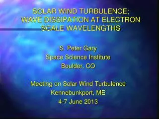
Spectrum of V; 0.3 AU, Helios 2, 6 days40.5 sec data. Slope = 1 (green)
Spectrum of V; 2 AU, Voyager 2, 8.3 hrs12 sec data; Slope = 1.5 (red), = 1.67 (green)
Spectrum of sqrt(rho)V, SW frame; 5 AU, Voyager 2, 44 days,96 sec data; Slope = 1.5 (red), = 1.67 (green)
B Current sheet Vsw q Inflow Boundary dB(q,f,t) & dv(q, f,t) are applied “Virtual Sun” Vsw Flux tubes: dBr(q,f); Velocity shear: dvr(q) Waves: dB(t) ||dv(t) f r The solutions described below were obtained in spherical coordinates in three dimensions, and at a resolution of 150150150 for r, , and
Br vs Bt simulated; 0.5 AU, initially Alfvénic but quickly evolving
Background • We use the "OMNI" 1-AU, combined hour-averaged solar wind dataset from J. King (NSSDC/SECAA) • 40 years of data exist, with 30 years complete enough for spectral analysis (~1/4 million points) • Here we examine magnetic and plasma quantities (B, V, B, n)
Overview • There is significant power at all scales from hours to 30 years, with high-frequency power laws and many spectral features at solar rotation, annual, and solar cycle frequencies. • The radial component of V dominates except at the smallest scales.
|B|: 11-year cycle; little 27-day power; multiple high-f power laws (Blue => 50pt smoothing) + –
Vr: 11-year and 27 day cycles; broad, high low-f power; -2 spectrum break to -5/3 + + B
Bt: Strong annual and 27-day peaks and harmonics (due to sectors); high-f power laws. + + + + + +
Br: 27-day and modulated (split) annual peak. Modulation is from 11/22-year cycle. ++
Ratio of energy in V to B; Dominant Vr, but all --> 0.5-1 at high-f; no “quasi-static” (“nonWKB”) region R N T
PVr/PVt; PVn/PVt; PBn/PBt: Dominant Vr and ~isotropic transverse components Vr/Vt Vn/Vt Bn/Bt
B ISEE-3, IMP-8, Interball
3-D, Q-2D + Slab, k-space; Fourier code initial condition kz ky kx “Slab”
Power Spectrum Correlation function 180 B^=(Bq2 + Bf2) f -180 0.5 1.82 r (AU) Shear produced 2-D correlation function, similar to solar wind observations B
Conclusions (1 of 2) • The minimum variance of B is nearly along B in highly Alfvénic regions; turbulence tends to decrease both effects. • |B| ~ const key to min variance (Barnes, 1981), and the “spherical polarization” follows the field. How? • WKB and simulations have failed to produce this effect; transverse variability is required, but how? • Compressive effects don’t help (Hollweg & Lilliequist, 1978). • The dominant energy in fluctuations from the scale of years to a fraction of a day is contained in the variation in the radial flow speed;
Conclusions (2 of 2) • There is no "quasi-static" regime for solar wind fluctuations but rather the transverse magnetic and velocity fluctuations are comparable in energy at essentially all scales. Why? • Neither quasi-2-D turbulence or slab waves will turn with the Parker field; only a nonlinear coupling of the two (or other means) will accomplish this. The “two component” model does not reflect this. • Shear can easily turn k, but not B. • Velocity and magnetic fluctuations evolve at different rates, and with different spectra. Turbulence theory?