Download
1 / 25
250 likes | 405 Views
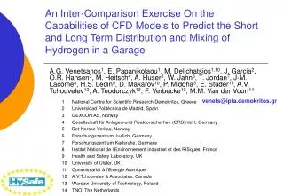
An Inter-Comparison Exercise On the Capabilities of CFD Models to Predict the Short and Long Term Distribution and Mixing of Hydrogen in a Garage. venets@ipta.demokritos.gr. 1 National Centre for Scientific Research Demokritos, Greece 2 Universidad Politécnica de Madrid, Spain

E N D
An Inter-Comparison Exercise On the Capabilities of CFD Models to Predict the Short and Long Term Distribution and Mixing of Hydrogen in a Garage venets@ipta.demokritos.gr 1 National Centre for Scientific Research Demokritos, Greece 2 Universidad Politécnica de Madrid, Spain 3 GEXCON AS, Norway 4 Gesellschaft für Anlagen-und Reaktorsicherheit (GRS)mbH, Germany 5 Det Norske Veritas, Norway 6 Forschungszentrum Juelich, Germany 7 Forschungszentrum Karlsruhe, Germany 8 Institut National de l’Environnement industriel et des RISques, France 9 Health and Safety Laboratory, UK 10 University of Ulster, UK 11 Commissariat à l’Energie Atomique 12 A.V.Tchouvelev & Associates, Canada 13 Warsaw University of Technology, Poland 14 TNO, The Netherlands A.G. Venetsanos1, E. Papanikolaou1, M. Delichatsios1,10, J. Garcia2, O.R. Hansen3, M. Heitsch4, A. Huser5, W. Jahn6, T. Jordan7, J-M. Lacome8, H.S. Ledin9, D. Makarov10, P. Middha3, E. Studer11, A.V. Tchouvelev12, A. Teodorczyk13, F. Verbecke10, M.M. Van der Voort14
Outline • Scope of work • SBEP-V3 specifications • SBEP-V3 participation • SBEP-V3 results • Evaluation methodology • Blind phase • Post phase • Conclusions
SBEPV3 Scope of work • To investigate for small hydrogen releases (<1g/s) within confined spaces on the phenomena occurring during the: • Release period (short term) • Diffusion period, i.e. long after the end of the release (long term) • To test the predictive ability of models/codes/organizations related to the above phenomena by performing • New experiments and in parallel • Blind simulations of the new experimental set • To develop consensus for the reasons of discrepancies between: • Different predictions using same models • Predictions of given models and experiment data • To improve our predictive ability by performing non-blind post calculations of the new experimental data
SBEPV3 Specifications Enclosure size: 7.2 x 3.78 x 2.88 m H2 mass flow rate: 1 g/s Nozzle diameter: 20 mm Exit velocity: 38.4 m/s Release duration: 240 s Test duration: 5400s Ambient temperature: 10 °C Target concentration: 3.53% Plastic sheet Release chamber Height 265mm Diameter: 120mm
SBEPV3 Participants • 12 HYSAFE partners: • CEA Commissariat à l’Energie Atomique, France • DNV Det Norske Veritas, Norway • FZJ Forschungszentrum Juelich, Germany • FZK Forschungszentrum Karlsruhe, Germany • GXC GEXCON AS, Norway • HSL Health and Safety Laboratory, UK • INERIS Institut National de l’Environement industriel et des RISques, France • NCSRD National Center for Scientific Research “Demokritos”, Greece • TNO Defence, Security and Safety Process Safety and Dangerous Goods, The Netherlands • UPM Universidad Politécnica de Madrid, Spain • UU University of Ulster, UK • WUT Warsaw University of Technology, Poland • 2 non-HYSAFE partners: • AVT A.V.Tchouvelev & Associates Inc., Canada • GRS Gesellschaft für Anlagen-und Reaktorsicherheit, Germany
SBEPV3 CFD codes • 10 CFD codes applied: • ADREA-HF • CAST3M • CFX 5.7.1 • CFX 10.0 • FDS 4.0 • FLACS 8.1 • FLUENT 6.2 • GASFLOW 2.4.12 • KFX • PHOENICS 3.6
SBEPV3 Turbulence models • 8 turbulence models applied: • Simple models • LVEL LVEL model • ML Generalized mixing length • Two equations models: • KE Standard k-ε • RNG RNG k- ε • REAL Realizable k- ε • SST SST model • LES models • Smagorinski subgrid • RNG subgrid
SBEPV3 Evaluation methodology Statistical measures: Mean relative bias Mean relative square error Averaging over all SBEP participant predictions for given sensor Predicted mean molar concentration (time averaged) Observed mean molar concentration (time averaged) Ideal values: Duijm et al. (1996) Journal of Loss Prevention in the Process Industry, Vol 9
SBEPV3 Blind Example prediction Release phase: 0-240s Diffusion phase: 240-5400s Blind prediction (NCSRD)
SBEPV3 Blind Release phase Large spread for sensors along the jet All sensors Large spread for sensors close to the ground and at large lateral distances from jet Time series averaging period 30-240 s
SBEPV3 Release Phase Comparison of data with existing correlations for sensors along jet axis Relatively good agreement Boussinesqu approximation overestimates concentrations Paranjpe (2004) Buoyant jets: Buoyant plumes: Chen and Rodi (1980)
SBEPV3 Blind Release phase LES-Smagorinski (Cs=0.2) too low mixing Sensor 16 Group of KE_GXC, KE_DNVa, KE_FZK SST_GRS, SST_HSL and INERIS data KE_DNV_b strangely high Group of KE_UPM, KE_NCSRD, KE_GRS RNG_AVT and REAL_WUT KE_FZJ strangely low LES-RNG too much mixing Mixing length too much mixing Group of LVEL_NCSRD and LVEL_AVT
SBEPV3 Blind Diffusion phase All sensors Mixing overestimated: higher concentrations close to the ground Mixing overestimated: Lower concentrations closer to the ceiling Time series averaging period 300-5400 s
SBEPV3 Blind Diffusion phase Sensor 12 Lower mixing is required Group of KE_GXC, KE_DNV_a, KE_FZJ
SBEPV3 Diffusion phase Average flammable cloud boundary Averaging time period 300-5400 s
SBEPV3 Blind Diffusion phase Risk assessment parameters Stratification. Group of LVEL_AVT, KE_FZK, KE_NCSRD, KE_GXC, KE_DNV_a, KE_FZJ, SST_HSL Too much mixing. Transition to homogeneous conditions. Group of LVEL_NCSRD, ML_CEA, KE_UPM, RNG_AVT, SST_GRS, VLES_UU
SBEPV3 Post Improvement steps • Numerical options • Grid • Improved vertical grid resolution • Some partners used the GEXCON grid • Time step • Reduced for both release and diffusion phases • Convective discretization scheme • Higher order schemes used • Physical models • LES • Smagorinski constant set to 0.1-0.12 • Turbulence switched manually off short after release • RNG_AVT and LVEL_AVT • Turbulent Schmidt number • Consistent use of the 0.7 value
SBEPV3 Post Release phase Sensor 16
SBEPV3 Release phase Averaging time period 30-240 s
SBEPV3 Diffusion phase Averaging time period 300-5400 s
SBEPV3 Conclusions Release phase • The effect of the turbulence model is clearly important. • In the jet region the standard k-ε model when applied without previous knowledge of the experimental data (blind prediction) generally tended to overestimate the concentrations. This was shown to be rectified either: • using a low turbulent Schmidt number (0.3) in combination with a first order upwind scheme or • using the usual value of 0.7 for turbulent Schmidt combined with a smaller time step and higher order convective scheme. • From the two approaches the second is recommended. • RNG k- ε and Realizable k- ε models showed tendency to overestimate the concentrations. • LVEL model generally tended to underestimate concentrations. • The SST model was found to produce hydrogen concentrations in the jet region lower than the standard k- model and in better agreement with the present experiment. • The LES Smagorinski model was found in good agreement with measured concentrations when the Smagorinski constant was set equal to 0.12
SBEPV3 Conclusions Diffusion phase • Experiments showed that a layer of hydrogen exists close to the ceiling, which is horizontally quasi homogeneous and vertically stratified. • Blind predictions showed two types of physical behaviour, either approximately constant stratification or fast transition to homogeneous hydrogen (non-flammable) distribution in the room. • Improvement of the predictions and reduction of spread between models was achieved in the post phase mainly by: • applying time step restrictions • reduction of vertical grid spacing • increase of the order of the convective scheme • The option of “manually” turning the turbulence model off although improved predictions in some cases cannot be suggested as a general recommendation. • Comparison between predicted and observed concentrations shows that the models generally tend to overestimate turbulent mixing Thank You Work funded by EC