Download
1 / 86
900 likes | 1.31k Views
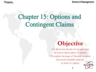
Chapter 15: Options and Contingent Claims. Objective To show how the law of one price may be used to derive prices of options To explore the range of financial decisions that can be fruitfully analyzed in terms of options. How Options Work Investing with Options

E N D
Chapter 15: Options and Contingent Claims • Objective • To show how the law of one price may • be used to derive prices of options • To explore the range of financial decisions • that can be fruitfully analyzed • in terms of options
How Options Work Investing with Options The Put-Call Parity Relationship Volatility & Option Prices Two-State Option Pricing Dynamic Replication & the Binomial Model The Black-Scholes Model Implied Volatility Contingent Claims Analysis of Corporate Debt and Equity Convertible Bonds Valuing Pure State-Contingent Securities Chapter 15 Contents
Terms • A option is the right (not the obligation) to purchase or sell something at a specified price (the exercise price) in the future • Underlying Asset, Call, Put, Strike (Exercise) Price, Expiration (Maturity) Date, American / European Option • Out-of-the-money, In-the-money, At-the-money • Tangible (Intrinsic) value, Time Value
Table 15.1 List of IBM Option Prices (Source: Wall Street Journal Interactive Edition, May 29, 1998) IBM (IBM) Underlying stock price 120 1/16 Put Call Strike Expiration Volume Last Open Volume Last Open Interest Interest 115 Jun 1372 7 4483 756 1 3/16 9692 115 Oct … … 2584 10 5 967 115 Jan … … 15 53 6 3/4 40 120 Jun 2377 3 1/2 8049 873 2 7/8 9849 120 Oct 121 9 5/16 2561 45 7 1/8 1993 120 Jan 91 12 1/2 8842 … … 5259 125 Jun 1564 1 1/2 9764 17 5 3/4 5900 125 Oct 91 7 1/2 2360 … … 731 125 Jan 87 10 1/2 124 … … 70
Table 15.2List of Index Option Prices (Source: Wall Street Journal Interactive Edition, June 6, 1998) S&P500 INDEX -AM Chicago Exchange Underlying High Low Close Net From % Change 31-Dec Change S&P500 1113.88 1084.28 1113.86 19.03 143.43 14.8 (SPX) Net Open Strike Volume Last Change Interest Jun 1110 call 2,081 17 1/4 8 1/2 15,754 Jun 1110 put 1,077 10 -11 17,104 Jul 1110 call 1,278 33 1/2 9 1/2 3,712 Jul 1110 put 152 23 3/8 -12 1/8 1,040 Jun 1120 call 80 12 7 16,585 Jun 1120 put 211 17 -11 9,947 Jul 1120 call 67 27 1/4 8 1/4 5,546 Jul 1120 put 10 27 1/2 -11 4,033
Call Put Terminal or Boundary Conditions for Call and Put Options 120 100 80 60 Dollars 40 20 0 0 20 40 60 80 100 120 140 160 180 200 -20 Underlying Price
The Put-Call Parity Relation • Two ways of creating a stock investment that is insured against downside price risk: • Buying a share of stock and a put option (a protective-put strategy) • Buying a pure discount bond with a face value equal to the option’s exercise price and simultaneously buying a call option
Terminal Conditions of a Call and a Put Option with Strike = 100 Share Call Put Share_Put Bond Call_Bond 0 0 100 100 100 100 10 0 90 100 100 100 20 0 80 100 100 100 30 0 70 100 100 100 40 0 60 100 100 100 50 0 50 100 100 100 60 0 40 100 100 100 70 0 30 100 100 100 80 0 20 100 100 100 90 0 10 100 100 100 100 0 0 100 100 100 110 10 0 110 100 110 120 20 0 120 100 120 130 30 0 130 100 130 140 40 0 140 100 140 150 50 0 150 100 150 160 60 0 160 100 160 170 70 0 170 100 170 180 80 0 180 100 180 190 90 0 190 100 190 200 100 0 200 100 200
Call_Bond Share_Put Bond Share Call Put 200 180 160 140 120 Payoffs 100 80 60 40 20 0 0 20 40 60 80 100 120 140 160 180 200 Stock Price
B: bond Put-Call Parity Equation
Synthetic Securities • The put-call parity relationship may be solved for any of the four security variables to create synthetic securities • C=S+P-B • S=C-P+B • P=C-S+B • B=S+P-C
Converting a Put into a Call • S = $100, E = $100, T = 1 year, r = 8%, P = $10: C = 100 – 100/1.08 + 10 = $17.41 • If C = $18, the arbitrageur would sell calls at a price of $18, and synthesize a synthetic call at a cost of $17.41, and pocket the $0.59 difference between the proceed and the cost
C=S+P-B Put-Call Arbitrage
or Options and Forwards • We saw in the last chapter that the discounted value of the forward was equal to the current spot • The relationship becomes If the exercise price is equal to the forward price of the underlying stock, then the put and call have the same price
Implications for European Options • If (F > E) then (C > P) • If (F = E) then (C = P) • If (F < E) then (C < P) • E is the common exercise price • F is the forward price of underlying share • C is the call price • P is the put price
Call = Put Strike = Forward
Put and Call as Function of Share Price 60 call 50 put asy_call_1 40 asy_call_2 asy_put_1 30 asy_put_2 Put and Call Prices 20 10 0 50 60 70 80 90 100 110 120 130 140 150 -10 Share Price 100/(1+r)
Strike PV Strike
Volatility and Option Prices P0 = $100, Strike Price = $100 Stock Price Call Payoff Put Payoff Low Volatility Case Rise 120 20 0 Fall 80 20 0 Expectation 100 10 10 High Volatility Case 0 Rise 140 40 Fall 60 0 40 Expectation 100 20 20 The prices of options increase with the volatility of the stock
Two-State Option Pricing: Simplification • The stock price can take only one of two possible values at the expiration date of the option: either rise or fall by 20% during the year • The option’s price depends only on the volatility and the time to maturity • The interest rate is assumed to be zero
Binary Model: Call • The synthetic call, C, is created by • buying a fraction x (which is called the hedgeratio) of shares, of the stock, S • selling short risk-free bonds with a market value y
Binary Model: Creating the Synthetic Call S = $100, E = $100, T = 1 year, d = 0, r = 0
Binary Model: Call • Specification: • We have an equation, and give the value of the terminal share price, we know the terminal option value for two cases: • By inspection, the solution is x=1/2, y = 40. The Law of One Price
Binary Model: Call • Solution: • We now substitute the value of the parameters x=1/2, y = 40 into the equation • to obtain
Binary Model: Put • The synthetic put, P, is created by • selling short a fraction x of shares, of the stock, S • buying risk free bonds with a market value y
Binary Model: Creating the Synthetic Put S = $100, E = $100, T = 1 year, d = 0, r = 0
Binary Model: Put • Specification: • We have an equation, and give the value of the terminal share price, we know the terminal option value for two cases: • By inspection, the solution is x = 1/2, y = 60 The Law of One Price
Binary Model: Put • Solution: • We now substitute the value of the parameters x=1/2, y = 60 into the equation • to obtain:
D $120 B $110 E $100 A $100 C $90 F $80 Decision Tree for Dynamic Replication of a Call Option
D $120 B $110 $20 E $100 C11 0 Decision Tree for Dynamic Replication of a Call Option • The terminal option value for two cases: • 120x – y = 20 • 100x – y = 0 • By inspection, the solution is x=1, y = $100 • Thus, C11= 1*$110 − $100 = $10
E $100 C $90 0 F $80 C12 0 Decision Tree for Dynamic Replication of a Call Option • The terminal option value for two cases: • 90x – y = 0 • 80x – y = 0 • By inspection, the solution is x=0, y = 0 • Thus, C12 = 0*$90 − $0 = $0
B $110 A $100 $10 C $90 C0 0 Decision Tree for Dynamic Replication of a Call Option • The terminal option value for two cases: • 110x – y = 10 • 90x – y = 0 • By inspection, the solution is x=1/2, y = $45 • Thus, C0= (1/2)*$100 − $45 = $5
D $120 B $110 E $100 A $100 C $90 F $80 Decision Tree for Dynamic Replication of a Call Option Sell shares $120 Pay off debt -$100 Total $20 Buy another half share of stock Increase borrowing to $100 Sell shares $100 Pay off debt -$100 Total 0 Buy 1/2 share of stock Borrow $45 Total investment $5 Sell stock and pay off debt
($120*100%) + (-$100) = $20 Decision Tree for Dynamic Replication of a Call Option
One can continuously and costlessly adjust the replicating portfolio over time As the decision intervals in the binomial model become shorter, the resulting option price from the binomial modelapproaches the Black-Scholes option price The Black-Scholes Model: The Limiting Case of Binomial Model
Bond Shares of Stock The Black-Scholes Model
C = price of call P = price of put S = price of stock E = exercise price T = time to maturity ln(·) = natural logarithm e = 2.71828... N(·) = cum. norm. dist’n The following are annual, compounded continuously: r = domestic risk free rate of interest d = foreign risk free rate or constant dividend yield σ = volatility The Black-Scholes Model: Notation
The Black-Scholes Model :Dividend-adjusted Form (Simplified)
Increases in: Call Put Stock Price, S Increase Decrease Exercise Price, E Decrease Increase Volatility, sigma Increase Increase Time to Expiration, T Ambiguous Ambiguous Interest Rate, r Increase Decrease Cash Dividends, d Decrease Increase Determinants of Option Prices
11 10 9 call put 8 7 6 Call and Put Price 5 4 3 2 1 0 1.0 0.9 0.8 0.7 0.6 0.5 0.4 0.3 0.2 0.1 0.0 Time-to-Maturity Value of a Call and Put Options with Strike = Current Stock Price
The value of σ that makes the observed market price of the option equal to its Black-Scholes formula value Approximation: S E r T d C σ 100 108.33 0.08 1 0 7.97 0.2 Implied Volatility
Insert any number to start Formula for option value minus the actual call value
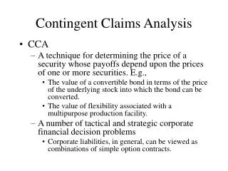
Valuation of Uncertain Cash Flows: CCA / DCF • The DCF approach discounts the expected cash flows using a risk-adjusted discount rate • The Contingent-Claims Analysis (CCA) uses knowledge of the prices of one or more related assets and their volatilities
An Example: Debtco Corp. • Debtco is in the real-estate business • It issues two types of securities: • common stock (1 million shares) • corporate bonds with an aggregate face value of $80 million (80,000 bonds, each with a face value of $1,000) and maturity of 1 year • risk-free interest rate is 4% • The total market value of Debtco is $100 million