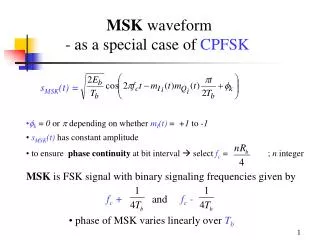
MSK Transmitter
m I (t). + +. S MSK (t). - +. m Q (t). . + +. cos(2 f c t ). . . cos( t/2T ). MSK Transmitter. (i) cos(2 f c t ) cos( t/2T ) 2 phase coherent signals at f c ¼R (ii) Separate 2 signals with narrow bandpass filters

MSK Transmitter
E N D
Presentation Transcript
mI(t) + + SMSK(t) - + mQ(t) + + cos(2fct) cos(t/2T) MSK Transmitter (i) cos(2fct)cos(t/2T) 2 phase coherent signals atfc ¼R (ii) Separate 2 signals with narrow bandpass filters (iii) Combined to formI & Q carrier components x(t), y(t) (iv) Mix and sum to yield SMSK(t) = x(t)mI(t) + y(t)mQ(t) mI(t) & mQ(t) = even & odd bit streams x(t) y(t)
Coherent MSK Receiver • (i) SMSK(t) split & multiplied by locally generated • x(t) & y(t) (I & Q carriers) • (ii) mixer outputs are integrated over 2T & dumped • (iii) integrate & dump output fed to decision circuit every 2T • input signal level compared to threshold decide 1 or 0 • output data streams correspond to mI(t) & mQ(t) • mI(t) & mQ(t) are offset & combined to obtain demodulated signal • *assumes ideal channel – no noise, interference
(2k+2)T 2kT (2k+1)T (2k-1)T SMSK(t) Coherent MSK Receiver Threshold Device mI(t) t = 2(k+1)T x(t) Switch At kT y(t) Threshold Device mQ(t) t = (2k+1)T
p(t) = PMSK(f) = MSK Power Spectrum • RF power spectrum obtained by frequency shifting |F{p(t)}|2 • F{} = fourier transform • p(t)= MSK baseband pulse shaping function (1/2 sin wave) Normalized PSD for MSK is given as
PSD of MSK & QPSK signals 10 0 -10 -20 -30 -40 -50 -60 QPSK, OQPSK MSK normalized PSD (dB) fc fc+0.5Rb fc+Rb fc+1.5Rb fc+2Rb • MSK spectrum • (1) has lower side lobes than QPSK (amplitude) • (2) has wider side lobes than QPSK (frequency) • 99% MSK power is within bandwidthB = 1.2/Tb • 99% QPSK power is within bandwidth B = 8/Tb
MSK • QPSK signaling is bandwidth efficient, achieving 2 bps per Hz of channel bandwidth. However, the abrupt changes results in large side lobes. Away from the main lobe of the signal band, the power spectral distribution falls off only as ω-2 . • MSK achieves the same bandwidth efficiency. With constant envelope (no discontinuity in phase), the power spectral distribution falls off as ω-4 away from the main signal band.
MSK spectrum • MSK has faster roll-off due to smoother pulse function • Spectrum of MSK main lobe > QPSK main lobe • - using 1st null bandwidth MSK is spectrally less efficient • MSK has no abrupt phase shifts at bit transitions • - bandlimiting MSK signal doesn’t cause envelop to cross zero • - envelope is constant after bandlimiting • small variations in envelope removed using hardlimiting • - does not raise out of band radiation levels • constant amplitude non-linear amplifiers can be used • continuous phase is desirable for highly reactive loads • simple modulation and demodulation circuits
Gaussian MSK • Gaussian pulse shaping to MSK • smoothens phase trajectory of MSK signal • over time, stabilizes instantaneous frequency variations • results in significant additional reduction of • sidelobe levels • GMSK detection can be coherent (like MSK) • or noncoherent (like FSK)
Gaussian MSK • premodulation pulse shaping filter used to filter NRZ data • - converts full response message signal into partial response scheme • full response baseband symbols occupy Tb • partial responsetransmitted symbols span several Tb • - pulse shaping doesn’t cause pattern’s averaged phase trajectory to deviate from simple MSK trajectory
Gaussian MSK • GMSKs main advantages are • power efficiency - from constant envelope (non-linear amplifiers) • excellent spectral efficiency • pre-modulation filtering introduces ISI into transmitted signal • if B3dbTb > 0.5 degradation is not severe • B3dB= 3dB bandwidth of Gaussian Pulse Shaping Filter • Tb= bit duration = baseband symbol duration • irreducible BER caused by partial response signaling is the • cost for spectral efficiency & constant envelope • GMSK filter can be completely defined from B3dB Tb • - customary to define GMSK by B3dBTb
Impulse responseof pre-modulation Gaussian filter : hG(t) = transfer function of pre-modulation Gaussian Filter is given by HG(f) = is related toB3dB by = Gaussian MSK
Impact of B3dBTb • (i) ReducingB3dBTb : spectrum becomes more compact (spectral efficiency) • causes sidelobes of GMSK to fall off rapidly • B3dBTb = 0.5 2nd lobe peak is 30dB below main lobe • MSK 2nd peak lobe is 20dB below main lobe • MSK GMSK with B3dBTb = • (ii) increases irreducible error rate (IER)due to ISI • ISI degradation caused by pulse shaping increases • however - mobile channels induce IER due to mobile’s velocity • if GMSK IER < mobile channel IER no penalty for using GMSK
0 -10 -20 -30 -40 -50 -60 BTb = (MSK) BTb = 1.0 BTb = 0.5 BTb = 0.2 0 0.5 1.0 1.5 2.0 (f-fc)T PSD of GMSK signals • Increasing BTb • reduces signal spectrum • results in temporal spreading and distortion
RF bandwidth containing % power as fraction of Rb e.g. for BT = 0.2 99% of the power is in the bandwidth of 1.22Rb • [Ish81] BER degradation from ISI caused by GMSK filtering is • minimal at B3dBTb= 0.5887 • degradation in required Eb/N0 = 0.14dB compared to case of no ISI
Pe = BER of GMSK for AWGN channel • [Mur81] shown to perform within 1dB of optimal MSK with B3dBTb = 0.25 • since pulse shaping causes ISI Peis function of B3dBTb Pe= bit error probability is constant related to B3dBTb • B3dBTb = 0.25 = 0.68 • B3dBTb = = 0.85 (MSK)
Gaussian LPF FM Transmitter RF GMSK Output NRZ bits GMSK Transmitter Block Diagram GMSK Transmitter • (i) pass mNRZ(t) through Gaussian base band filter (see figure below) • - mNRZ(t) = NRZ bit stream • output of Gaussian filter passed to FM modulator • used in digital implementation for • - Global System for Mobile (GSM) • - US Cellular Digital Packet Data (CDPD) • (ii) alternate approach is to use standard I/Q modulator
demodulated signal /2 modulated IF input signal loop filter Q IF LO I /2 clock recovery • GMSK Receiver • RF GMSK signal can be detected using • (i) orthogonal coherent detectors (block diagram) • (ii) simple non-coherent detectors (e.g. standard FM discriminators) (i) GMSK Receiver Block Diagram-orthogonal coherent detectors
carrier recovery using De Budas method for(similar to Costas loop) • S’(t) = output of frequency doubler that contains 2 discrete frequency • components • - divide S’(t) by four: S’(t) /4 • - equivalent to PLL with frequency doubler
D Q C D Q C D Q C D Q C modulated IF input signal D Q C clock recovery demodulated signal D C Q loop filter VCO • De Budasmethod implemented using digital logic • 2 D flip flops (DFF) act as quadrature product demodulator • XORs act as based band multipliers • mutually orthogonal reference carriers generated using 2 DFFs • VCOcenter frequency set to 4 fc ( fc = carrier center frequency) Logic Circuit for GMSK demodulation
Orthogonal Frequency Shift Keying (FSK)Review • If there are two frequencies for FSK: ω1 , ω2 , • one may use a carrier frequency: ωc = (ω1 + ω2)/2 , • then the two frequencies are: • ω1 , ω2 = ωc± (ω2 – ω1)/2 • For OFSK, the minimum frequency separation is • (ω2 – ω1)T = π • Therefore • ω1 , ω2 = ωc±π/(2T)
Orthogonal Frequency Shift Keying (FSK)Review • With the two frequencies in OFSK written as: • ω1 , ω2 = ωc± (ω2 – ω1)/2 = ωc± π/(2T), • the signals may be written as: • cos ωit = cos {ωct ± πt/(2T)}, • which may be interpreted as • modulating the the carrier: cos ωct • with linear change in phase of ±πt/(2T). • This phase change relative to the carrier • is shown in the figure. π/2 t 0 T -π/2 d0
Orthogonal Frequency Shift Keying (FSK)with binary data stream • We now generalize to the case for a binary data stream: d0 , d1, d2 for which dk = ±1. • The signals at kT < t < (k+1)T for OFSK with coherent detection can be written as • s(t)/(2E/T)1/2 = cos[{ωc + dkπ/(2T)}t + γk], • where γk is constant during the time kT < t < (k+1)T • The value of γk in each value of k will be chosen in order to make the phase continuous at the boundaries between adjacent samples.
Orthogonal Frequency Shift Keying (FSK) • Frequencies: ωc±π/(2T); tone spacing: π/T • In each time interval kT < t < (k+1)T, the phase changes by ±π/2 • The slope of this phase shift versus time is the frequency shift from ωc by ±π/(2T). • This frequency shift from ωc may also be viewed as a linear phase shift of dkπt/(2T) relative to the carrier. dk=1: dashed line dk=-1: dotted line π/2 dkπt/(2T) 0 T 2T 3T 4T 5T 6T 7T 8T -π/2 d0
CPFSKPhase continuity at the boundaries t=kT • We are now going to remove phase discontinuity of OFSK at the sampling time boundaries • t = kT • by choosing the appropriate values of the γk term in • s(t)/(2E/T)1/2 = cos[{ωc + dkπ/(2T)}t + γk] . • We first note that • Difference between adjacent bits is dk – dk-1 = 0 or ±2 • Product of adjacent bits is dk dk-1 = ±1
Phase continuity at the boundaries t=kT • We start at k=0 • The phase term d0πt/(2T) = 0 at t=0, and is therefore continuous here. • We therefore choose γ0 – γ-1 = 0 • The phase term at t=T may then take the values ±π/2 dk=1: dashed line dk=-1: dotted line π dkπt/(2T) π/2 0 T 2T 3T 4T 5T 6T 7T 8T -π/2 -π d0
Phase continuity at the boundaries t=kTTrellis diagram • At k = 1, if d1 – d0 = 0 (d1 d0 = +1), the d1πt/(2T) term is continuous with the d0πt/(2T) term at t=T. • We therefore choose γ1 – γ0 = 0 dk=1: dashed line dk=-1: dotted line π dkπt/(2T) π/2 0 T 2T 3T 4T 5T 6T 7T 8T -π/2 -π d0
Phase continuity at the boundaries t=kTTrellis diagram • At k = 1, if d1 – d0 = ±2 (d1 d0 = -1), • d1πt/(2T) – d0πt/(2T) = ±π at t=T. • We therefore choose γ1 – γ0 = π to remove the phase discontinuity. dk=1: dashed line dk=-1: dotted line π π dkπt/(2T) π/2 π/2 0 T 2T 0 T 2T -π/2 -π/2 -π -π d0 d0
Phase continuity at the boundaries t=kTTrellis diagram • In summary, γ1 – γ0 = {(1 – d1 d0)/2} π • = 0 if d1 d0 = +1 • = 1 if d1 d0 = –1. • Then d1πt/(2T) = 0, ±π at t=T. dk=1: dashed line dk=-1: dotted line π dkπt/(2T) π/2 0 T 2T 3T 4T 5T 6T 7T 8T -π/2 -π d0
Phase continuity at the boundaries t=kTTrellis diagram • At k=2, d2πt/(2T) = 0, ±π at t=T. • The d2πt/(2T) = 0 case is same as that at k=0. • The d2πt/(2T) = ±π cases are considered next. dk=1: dashed line dk=-1: dotted line π dkπt/(2T) π/2 0 T 2T 3T 4T 5T 6T 7T 8T -π/2 -π d0
Phase continuity at the boundaries t=kTTrellis diagram • At k=2, if d2πt/(2T) = ±π at t=2T and d2 d1 = +1 • d2πt/(2T) – d1πt/(2T) = 0 so that the phase is continuous. dk=1: dashed line dk=-1: dotted line π dkπt/(2T) π/2 0 T 2T 3T 4T 5T 6T 7T 8T -π/2 -π d0
Phase continuity at the boundaries t=kTTrellis diagram • Cases of k=2, d2πt/(2T) = ±π at t=2T and d2 d1 = +1: • Because cosine is periodic, we can show it with shifts of 2π to the phase without affecting the value of cosine. • γ2 – γ1 = {(1 – d2 d1)/2} 2π = integer multiple of 2π dk=1: dashed line dk=-1: dotted line π dkπt/(2T) π/2 0 T 2T 3T 0 T 2T 3T -π/2 -π d0 d0
Phase continuity at the boundaries t=kTTrellis diagram • If d2 d1 = -1, the terms d2πt/(2T) and d1πt/(2T) differ by 2π so that cosine function is still continuous • γ2 – γ1 = {(1 – d2 d1)/2} 2π = integer multiple of 2π dk=1: dashed line dk=-1: dotted line π dkπt/(2T) π/2 0 T 2T 3T 0 T 2T 3T -π/2 -π d0 d0
Phase continuity at the boundaries t=kTTrellis diagram • All the different scenarios for 2T<t<3T are shown: • γ2 – γ1 = {(1 – d2 d1)/2} 2π = integer multiple of 2π • Owing to periodicity, only 5 different states (0, ±π/2, ±π) need to be shown in the Trellis diagram. π dkπt/(2T) π/2 0 0 T 2T 3T -π/2 dk=1: dashed line dk=-1: dotted line -π d0
Phase continuity at the boundaries t=kTTrellis diagram • The possible values of the phase at t=3T are the same as those at t=T. • Therefore the Trellis diagram for 3T<t<5T is the same as that for T<t<3T. • That is, the Trellis diagram is repeating itself every 2T. π dkπt/(2T) π/2 0 T 2T 3T 4T 5T dk=1: dashed line dk=-1: dotted line -π/2 -π d0
Phase continuity at the boundaries t=kTTrellis diagram • When k =2j, the d2jπt/(2T) term is continuous. Therefore γ2j – γ2j-1 ={(1 – d2j d2j-1)/2} 2jπ = integer multiple of 2π π dkπt/(2T) π/2 0 T 2T 3T 4T 5T 6T 7T 8T -π/2 -π dk=1: dashed line dk=-1: dotted line d0
Phase continuity at the boundaries t=kTTrellis diagram • When k =2j+1 and d2j+1 d2j = 1, also γ2j+1 – γ2j = 0 • When k =2j+1 and d2j+1 d2j = –1, the d2j+1πt/(2T) term changes by ±π. Therefore γ2j+1 – γ2j = π • γ2j+1 – γ2j ={(1 – d2j+1 d2j)/2}(2j+1)π = odd multiple of π π dkπt/(2T) π/2 0 T 2T 3T 4T 5T 6T 7T 8T -π/2 -π dk=1: dashed line dk=-1: dotted line d0
Continuous Phase FSK • s(t)/(2E/T)1/2 • = cos{ωct + d2jπt/(2T) + γ2j-1}, when k=2j • = cos{ωct + d2j+1πt/(2T) + γ2j + (1–d2j+1d2j)π/2}, • when k=2j+1
Continuous Phase FSK • s(t)/(2E/T)1/2 • = cos{ωct + d2jπt/(2T) + γ2j-1} • = (-1)(γ2j-1)/π cos{ωct + d2jπt/(2T)}, when k=2j ; • = cos{ωct + d2j+1πt/(2T) + γ2j + (1–d2j+1d2j)π/2} • = (-1)(γ2j)/π cos{ωct + d2j+1πt/(2T) + (1–d2j+1d2j)π/2}, when k=2j+1 .
MSK from CPFSKk=2j+1 • When k=2j+1, • s(t)/(2E/T)1/2 • = (-1)(γ2j)/π cos{ωct + d2j+1πt/(2T) + (1–d2j+1d2j)π/2} • = d2j+1d2j (-1)(γ2j)/π cos{ωct + d2j+1πt/(2T) + γ2j} • because • s(t)/(2E/T)1/2 = cos{ωct + d2j+1πt/(2T) + γ2j} • if d2j+1d2j = 1 • = – cos{ωct + d2j+1πt/(2T) + γ2j} • if d2j+1d2j = -1
MSK from CPFSK • s(t)/(2E/T)1/2 • = (-1)(γ2j-1)/π cos{ωct + d2jπt/(2T)} when k=2j • = d2j+1d2j (-1)(γ2j)/π cos{ωct + d2j+1πt/(2T)} when k=2j+1
MSK from CPFSK • s(t)/(2E/T)1/2 • = (-1)(γ2j-1)/π cos{ωct + d2jπt/(2T)} when k=2j • = d2j+1d2j (-1)(γ2j)/π cos{ωct + d2j+1πt/(2T)} when k=2j+1 • As FSK, its frequency is ωct + 2π dk/(4T) • As CPFSK, it also contains a history dependent phase term that makes the phase continuous at the sampling time boundaries.
CPFSK versus Offset QPSKk=2j • When k=2j, • s(t)/(2E/T)1/2 = (-1)(γ2j-1)/π cos{ωct + d2jπt/(2T)} • = (-1)(γ2j-1)/π • [cos{d2jπt/(2T)} cos(ωct) – sin{d2jπt/(2T)} sin(ωct)] • = (-1)(γ2j-1)/π • [cos{πt/(2T)} cos(ωct) – d2jsin{πt/(2T)} sin(ωct)] • where the modulation d2jsin{πt/(2T)} is on the Q component sin(ωct).
CPFSK versus Offset QPSKcos [{(ωc±π/(2T)}t] formula • d2j = –1: cos [{(ωc – π/(2T)}t] • = cos(ωct) cos{πt/(2T)} + sin(ωct) sin{πt/(2T)}
CPFSK versus Offset QPSKcos [{(ωc±π/(2T)}t] formula • d2j = –1: cos [{(ωc – π/(2T)}t] • = cos(ωct) cos{πt/(2T)} + sin(ωct) sin{πt/(2T)} • = cos(ωct) cos{πt/(2T)} + cos(ωct – π/2) sin{πt/(2T)} • In the region 2jT<t<(2j+1)T (e.g., 0<t<T): • near t=0, the sum ≈cos(ωct) • near t=T, the sum ≈cos(ωct – 2π/4) • The phase is retarded by 2π/4 per ωcT, • which is equivalent to decreasing carrier frequency by 1/4T
CPFSK versus Offset QPSKcos [{(ωc±π/(2T)}t] formula • d2j = +1: cos [{(ωc + π/(2T)}t] • = cos(ωct) cos{πt/(2T)} – sin(ωct) sin{πt/(2T)}
CPFSK versus Offset QPSKcos [{(ωc±π/(2T)}t] formula • d2j = +1: cos [{(ωc + π/(2T)}t] • = cos(ωct) cos{πt/(2T)} – sin(ωct) sin{πt/(2T)} • = cos(ωct) cos{πt/(2T)} + cos(ωct + π/2) sin{πt/(2T)} • In the region 2jT<t<(2j+1)T (e.g., 0<t<T): • near t=0, the sum ≈cos(ωct) • near t=T, the sum ≈cos(ωct + 2π/4) • The phase is advanced by 2π/4 per ωcT, • which is equivalent to increasing carrier frequency by 1/4T
CPFSK versus Offset QPSKk=2j • When k=2j, • s(t)/(2E/T)1/2 = (-1)(γ2j-1)/π cos{ωct + d2jπt/(2T)} • = (-1)(γ2j-1)/π • [cos{πt/(2T)} cos(ωct) – d2jsin{πt/(2T)} sin(ωct)] • In the region 2jT<t<(2j+1)T, put t=2jT+t’, i.e., 0<t’<T: • d2jsin{πt/(2T)} = d2jsin{jπ+πt’/(2T)} • = (-1)j d2jsin{πt’/(2T)}
CPFSK versus Offset QPSKk=2j+1 • When k=2j+1, • s(t)/(2E/T)1/2 = (-1)(γ2j-1)/π d2j+1d2j cos{ωct + d2j+1πt/(2T)} • = d2j+1d2j (-1)(γ2j-1)/π • [cos{d2j+1πt/(2T)} cos(ωct) – sin{d2j+1πt/(2T)} sin(ωct)] • = d2j+1d2j (-1)(γ2j-1)/π • [cos{πt/(2T)} cos(ωct) – d2j+1 sin{πt/(2T)} sin(ωct)] • = d2j (-1)(γ2j-1)/π • [d2j+1 cos{πt/(2T)} cos(ωct) – sin{πt/(2T)} sin(ωct)] • where the modulation d2j+1cos{πt/(2T)} is on the I component cos(ωct)
CPFSK versus Offset QPSKk=2j+1 • When k=2j+1, • s(t)/(2E/T)1/2 = (-1)(γ2j-1)/π d2j+1d2j cos{ωct + d2j+1πt/(2T)} • = d2j (-1)(γ2j-1)/π • [d2j+1 cos{πt/(2T)} cos(ωct) – sin{πt/(2T)} sin(ωct)] • In the region (2j+1)T<t<(2j+2)T, put t=(2j+1)T+t’, i.e., 0<t’<T: • d2j+1cos{πt/(2T)} = d2j+1cos{π(2j+1)/2} +πt’/(2T)} • = –(-1)j d2j+1sin{πt’/(2T)}
CPFSK versus Offset QPSK • The I- and Q-components are each of the form: • data-dependent term * sinusoidal symbol weighting * carrier • The cos{πt/(2T)} and sin{πt/(2T)} are sinusoidal symbol weighting. • The cos(ωct) and sin(ωct) are the carrier.