Selection and Drift in Ecological Communities: Understanding Coexistence Mechanisms
230 likes | 383 Views
This text explores the dynamics of selection and drift within ecological communities, using theoretical frameworks like Lotka-Volterra competition models and Chesson’s mechanisms. It discusses the conditions under which species can coexist, based on fitness and niche differences. The balance of factors such as selection coefficients and community size can influence species dynamics, leading to stable or unstable equilibrium points. Key insights from past studies on resource use, community diversity, and frequency dependency provide a nuanced understanding of ecological interactions.

Selection and Drift in Ecological Communities: Understanding Coexistence Mechanisms
E N D
Presentation Transcript
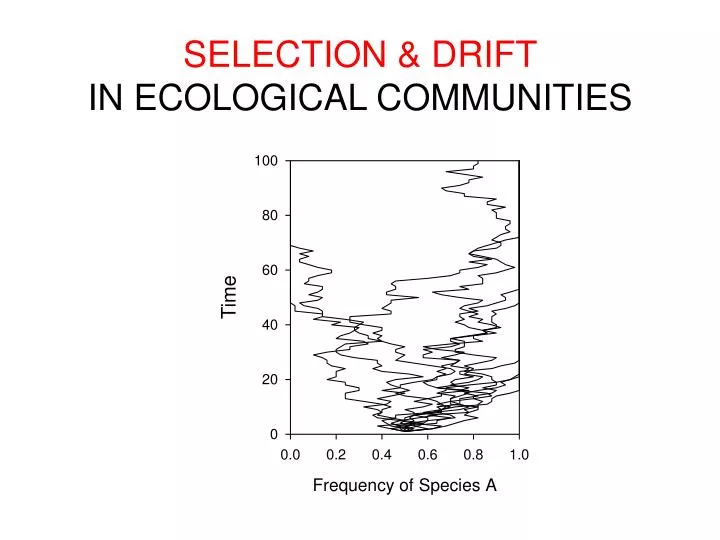
SELECTION & DRIFT IN ECOLOGICAL COMMUNITIES Time
In the beginning… We always had selection: Per capita competitive effect of sp. 2 on sp. 1 a11N1 + a12N2 K1 = r1N11 - dN1 dt Lotka-Volterra competition
If aij < 1, stable coexistence possible K1/a12 K2 N2 K2/a21 K1 N1
The Community Matrix (Levins 1968) 1 2 3 4 5 Species 1 2 3 4 5 Species
Some stuff people said based on analyses of this type of model: • There is a limit to the similarity in resource use between coexisting species (MacArthur & Levins 1967) • Diversity (i.e., more species) destabilizes a community (May 1972) • All based on analysis of equilibrium points in deterministic models; focus on species differences
But there’s more than one way to be “different”… “Fitness” differences: ri > rj, Ki > Kj If large, coexistence less likely “Niche” differences: aij < 1 If large, coexistence more likely a11N1 + a12N2 K1 = r1N11 - dN1 dt a22N2 + a21N1 K2 = r2N21 - dN2 dt
Fitness difference between species i and community average small fitness differences Formalization in Chesson’s “Equalizing” vs. “Stabilizing” mechanisms of coexistence large niche differences Coexistence happens when each species tends to increase in relative abundance when rare, so… Niche difference(1 – overlap) Population growth rate when rare for species i Chesson (2000, Ann. Rev. Ecol. Syst)
Bottom line: A big fitness difference means you need a big niche difference for coexistence (and vice versa) Niche difference(1 – overlap) Fitness difference between species i and community average Population growth rate when rare for species i Chesson (2000, Ann. Rev. Ecol. Syst)
expected dynamics (sp. A wins) stable equilibrium unstable equilibrium A simpler way to think about it (I think)… FORMS OF SELECTION BETWEEN TWO SPECIES, A & B A. Constant selection + FitnessA – FitnessB 0 - 0 1 Frequency of Species A
stable equilibrium + + + + unstable equilibrium D. Complex frequency-dependence - - - - B. Negative frequency-dependence E. Neutral C. Positive frequency-dependence FORMS OF SELECTION BETWEEN TWO SPECIES A. Constant + - FitnessA – FitnessB Frequency of Species A
only a little a lot + + - - Equalizing and Stabilizing Mechanisms of CoexistenceHow much do you need to bend these lines (while maintaining average height) to get stable coexistence? Fitness difference large Fitness difference small + + - - FitnessA – FitnessB
+ - only a little a lot + + - - Equalizing and Stabilizing Mechanisms of CoexistenceHow much do you need to raise these lines (while maintaining bendiness) to get rid of stable coexistence? Niche difference large Niche difference small + - FitnessA – FitnessB Prone to the influence of drift
Combining selection and drift(Starting with pure drift) # NEUTRAL MODEL (single community, no speciation) # Set initial community (e.g., 25 individuals of sp. 1 + 25 of sp. 2; J = 50) J <- 50 # must be an even number COM <- vector(length=J) COM[1:J/2] <- 1 COM[(J/2+1):J] <- 2 # set number of “years” to run simulations & empty matrix for data num_years <- 50 prop_1 <- matrix(0,nrow=J*num_years,ncol=1) # run model for (i in 1:(J*num_years)) { COM[ceiling(J*runif(1))] <- COM[ceiling(J*runif(1))] prop_1[i] <- sum(COM[COM==1])/J } # plot results plot(prop_1, type="l")
Combining selection and drift # SELECTION-DRIFT MODEL (single community, no speciation) # Set initial community (e.g., 25 individuals of sp. 1 + 25 of sp. 2; J = 50) J <- 50 # must be an even number COM <- vector(length=J) COM[1:J/2] <- 1 COM[(J/2+1):J] <- 2 s <- 0.02 # the selection coefficient # set number of “years” to run simulations & empty matrix for data num_years <- 50 prop_1 <- matrix(0,nrow=J*num_years,ncol=1) prop_1 <- 0.5 # run model for (i in 2:(J*num_years)) { death_cell <- ceiling(J*runif(1)) prob_1 <- (1+s)*prop_1[i-1] if (runif(1) < prob_1) COM[death_cell] <- 1 else COM[death_cell] <- 2 prop_1[i] <- sum(COM[COM==1])/J } # plot results plot(prop_1, type="l")
Selection makes some outcomes more likely than others, but it does not guarantee any particular outcome
An example of bringing together drift & selection:Effects of finite community size on invasion probabilities The analogies: new mutation = new species selection coefficient, s = population growth rate, r effective population size, Ne = effective community size, Je initial frequency of allele/species = p From Kimura (1962): Pr(inv) = (1 – exp(-2Jerp)) / (1 – exp(-2Jer)) Vellend & Orrock (2010, In: Theory of Island Biogeography Revisited
From Kimura (1962): Pr(inv) = (1 – exp(-2Jerp)) / (1 – exp(-2Jer)) Key (obvious) results: Invasion more likely with higher r Invasion more likely with higher p But how does Je (i.e., drift) modulate these effects? Vellend & Orrock (2010, In: Theory of Island Biogeography Revisited
For a given initial frequency, invasion less likely in small communities 0.9 0.8 0.7 r = 0.01, J = 1000 0.6 Invasion Probability Pr(inv) 0.5 0.4 0.3 0.2 r = 0.01, J = 100 0.1 0.0 0.12 0 0.02 0.04 0.06 0.08 0.1 Initial frequency, p = Ninit/J Vellend & Orrock (2010, In: Theory of Island Biogeography Revisited
For a given initial population size, invasion more likely in small communities 0.20 Ninit = 5 0.15 Invasion Probability Pr(inv) J = 100 0.10 J = 1000 0.05 0.00 0.000 0.005 0.010 0.015 0.020 Population growth rate, r Vellend & Orrock (2010, In: Theory of Island Biogeography Revisited
B. Introduced species Frequency Pop. growth rate when rare, r Wild speculations A. Mutations Lethal Frequency From Hedrick (2000) Selection coefficient, s
Invader is superior Invader is inferior Based on the Kimura equations…
Other selection-drift models for communities… Stochastic Niche Theory: “Classic” Tilman with some stochasticity Invasion (establishment) modeled probabilistically based on small initial population that might to extinct (demographic stochasticity) despite being deterministically favored Resource competition with environmental (temperature) heterogeneity
Other selection-drift models for communities (this one with dispersal)…