Download
1 / 48
480 likes | 618 Views
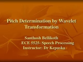
Pitch Determination by Wavelet Transformation Santhosh Bellikoth ECE 5525- Speech Processing Instructor: Dr Kepuska . Pitch Determination. Equivalent to fundamental frequency estimation Essential Component in all Speech Processing system. Applications of Pitch Detector.

E N D
Pitch Determination by Wavelet TransformationSanthosh Bellikoth ECE 5525- Speech Processing Instructor: Dr Kepuska
Pitch Determination • Equivalent to fundamental frequency estimation • Essential Component in all Speech Processing system
Applications of Pitch Detector • Speaker Identification and Verification • Pitch Synchronous speech analysis and Synthesis • Linguistic and phonetic knowledge acquisition • Voice disease diagnosis
Continuous Wavelet transform • Continuous Wavelet transform is defined as the convolution of a signal x (t) with a wavelet functionΨ(t) shifted in time by a translation parameter ‘b‘ and a dilation parameter ‘a’
Dyadic Wavelet Transform • Dyadic Wavelet Transform is defined as
Dyadic Wavelet Transform Properties • Linearity • Time Shift Variance • Detection of sharp and slow variation in the signal, which makes it useful tool for the analysis of Speech Signal.
Pitch Detection Steps • Segmentation of Speech Signal • Scale Selection • Computation of Wavelet Transformation of each frame at various scales • Locating Position of local maxims for each frame • Locating position of GCIs • Calculation of Pitch Periods
Segmentation of Speech Signal 1) Segmentation without Overlapping Speech Signal is segmented using a hamming window of 40 ms duration 2) Segmentation with 50 % Overlapping Rectangular window is used with overlapping of less than 10 %
Scale Selection • Dyalet Wavelet Transform is computed at scales a=2^j for all j. • Number of Scales for computation of can be reduced based on the nature of the speech signal.
Number of Scales Selection • Wavelet with input center frequency fci and input bandwidth Δfi, Scale parameter ‘a’ corresponding to the required output center frequency fco using the following relation a= fci/fco
Input and Output bandwidth • Input bandwidth of the wavelet Δfi= 2*fci • Output Bandwidth of the wavelet Δfo=2*fco
Approximation of ‘a’ • If fci/fco is not to some power of 2, then it is rounded off to nearest power • For high pitch speakers lower bound is decreased and upper bound is increased for the better results
Computation of Dyadic Wavelet Transform • The Dyadic Wavelet Transform is computed for each frame by the following equation
First Three Frames of Original Speech Signal with 50% overlapping
Locating Positions of Local maxims • For locating the position of local maxims, first all the peaks of the waveform are located. • Positions of local maxims are computed by setting a threshold, which is 80% of the global maximal.
Locating all the upside peaks of a waveform and local maxims
Locating the position of GCI’s (Glottal closure Instant) • If the position of local maxima at a scale matches the position of local maxima of frame whose wavelet transform has been calculated, then those locations are called GCI’s position • If it does not match then it is compared with the Wavelet transform at next higher scale
Pitch Calculation • Pitch can be computed as d is the difference between two GCI positions in terms of sample and fs is the sampling frequency of the speech signal
Acoustic Measures • Jita Jita is absolute Jitter, which gives an evaluation in msec of the period to period variability of the Pitch period with in the analyzed voice sample
Jitter • Jitter percent gives an evaluation of the variability of the pitch period within the analyzed voice sample in percent. P is the pitch period and N is the number of pitch estimated.
Shimmer (DB) • Shimmer in dB gives an evaluation of the period to period variability of the peak to peak amplitude within the analyzed voice sample.
Shimmer(%) • Shimmer percent gives an evaluation in percent of the variability of the peak to peak amplitude within the analyzed voice sample. Shimmer in percent is given by
Conclusion • Acoustic parameters computed using wavelet transform can be used for the objective analysis of pathological voice. • These Acoustic parameters can be used to differentiate between normal and pathological voice.
Final Program • clc; • clear all; • close all; • [s,fs]=wavread('U:\speech2_10k.wav'); %s=s1(1:10000); • m=400; • wL=400; • L=length(s); • nf=floor(L/wL); • j=1; • t=10;
Final program • cmp1=[]; • cmp2=[]; • cmp3=[]; • gci=[]; • q=[]; • d=[]; • a=[]; • %b=[]; • disp('Enter x=1 for male voice'); • disp('Enter x=2 for female voice');
Final Program • x=input('Enter the value of x ='); • switch x • case 1 • for i=1:nf-1 • f(j,:)=f_ovp(s,m,wL,i); • g=gne(f(j,:)); • c1=cwt(f(j,:),4,'haar'); • c2=cwt(f(j,:),8,'haar'); • c3=cwt(f(j,:),16,'haar'); • c4=cwt(f(j,:),32,'haar');
Final Program • [p1,q1,d1]=f_shim_max(c1); • [p2,q2,d2]=f_shim_max(c2); • [p3,q3,d3]=f_shim_max(c3); • [p4,q4,d4]=f_shim_max(c4); • L1=length(p1); • L2=length(p2); • L3=length(p3); • L4=length(p4); • if L1==L2 • cmp1=comp_t(p1,p2,t);
Final Program • elseif L2==L3 • cmp2=comp_t(p2,p3,t); • elseif L3==L4 • cmp3=comp_t(p3,p4,t); • end • if ~isempty(cmp1) • gci=[gci,p1']; • q=[q,q1']; • d=[d,d1']; • elseif ~isempty(cmp2)
Final Program • gci=[gci,p2']; • q=[q,q2']; • d=[d,d2']; • elseif ~isempty(cmp3) • gci=[gci,p3']; • q=[q,q3']; • d=[d,d3']; • elseif isempty(cmp1)& isempty(cmp2) • d=[d,zeros(1,1)]; • end
Final Program • end • a=[a g]; • % b=[b g2]; • j=j+1; • end • %d1=diff(gci); • case 2 • for i=1:nf-1 • f(j,:)=f_ovp3t(s,m,wL,i); • c1=cwt(f(j,:),8,'haar'); • c2=cwt(f(j,:),16,'haar'); • c3=cwt(f(j,:),32,'haar'); • c4=cwt(f(j,:),64,'haar'); • g=gne(f(j,:)); • [p1,q1,d1]=f_shim_max(c1); • [p2,q2,d2]=f_shim_max(c2);
Final Program • [p3,q3,d3]=f_shim_max(c3); • [p4,q4,d4]=f_shim_max(c4); • L1=length(p1); • L2=length(p2); • L3=length(p3); • L4=length(p4); • if L1==L2 • cmp1=comp_t(p1,p2,t); • elseif L2==L3 • cmp2=comp_t(p2,p3,t); • elseif L3==L4 • cmp3=comp_t(p3,p4,t); • end • if ~isempty(cmp1) • gci=[gci,p1'];
Final Program • q=[q,q1']; • d=[d,d1']; • elseif ~isempty(cmp2) • gci=[gci,p2']; • q=[q,q2']; • d=[d,d2']; • elseif ~isempty(cmp3) • gci=[gci,p3']; • q=[q,q3']; • d=[d,d3']; • elseif isempty(cmp1)& isempty(cmp2) • d=[d,zeros(1,1)]; • end • a=[a g]; • % b=[b g2];
Final Program • d=smooth_d(d); • p=d./fs; • L5=length(gci); • L6=length(p); • L7=abs(L5-L6); • m=mean(p); • fo=1/m; • m1=max(p); • m2=min(f_wz(p)); • fh=1/m2; • fl=1/m1; • jit=jita(p); • jitt=jitter(p); • shdB=shimdB(q,L6); • sh=shimmer(q,L6); • GNE=max(a);
Final Program • %GNE2=max(b); • disp('Fundamental frequency ='); • disp(fo); • disp('Highest frequency='); • disp(fh); • disp('Lowest frequency='); • disp(fl); • disp('Jita ='); • disp(jit); • disp('Jitter in percentage'); • disp(jitt); • disp('Shimmer in dB ='); • disp(shdB); • disp('shimmer in percentage='); • disp(sh);
Final Program • disp('Press any key for plot'); • pause; • if L5==L6 • stairs(gci,p); • xlabel('Number of Samples'); ylabel('Pitch period in msec'); title('Pitch contour'); • elseif L5<L6 • gci=[gci,zeros(1,L7)]; • stairs(gci,p); • xlabel('Number of Samples'); ylabel('Pitch period in msec'); title('Pitch contour'); • else • p=[p,zeros(1,L7)]; • stairs(gci,p); • xlabel('Number of Samples'); ylabel('Pitch period in msec'); title('Pitch contour'); • end
Results and Observations • Enter x=1 for male voice • Enter x=2 for female voice • Enter the value of x =1 • Fundamental frequency = • 351.4493 • Highest frequency= • 3.3333e+003 • Lowest frequency= • 217.3913 • Jita = • 0.0021 • Jitter in percentage • 72.4864
Results and observations • Jitter in percentage • 72.4864 • Shimmer in dB = • 3.2017 • shimmer in percentage= • 15.6931 • Press any key for plot • >> • Variables created in current workspace. • Variables created in current workspace. • >>