Download
1 / 55
590 likes | 814 Views
Network Address Translation ✧ Inside Internet Routers. GZ01 Networked Systems Kyle Jamieson Lecture 7 Department of Computer Science University College London. Today. Network address translation (NAT) Inside internet routers Architecture Crossbar scheduling: iSLIP algorithm

E N D
Network Address Translation✧Inside Internet Routers GZ01 Networked Systems Kyle Jamieson Lecture 7 Department of Computer Science University College London
Today • Network address translation (NAT) • Inside internet routers • Architecture • Crossbar scheduling: iSLIP algorithm • Longest-prefix lookup: Luleå algorithm
Network Address Translation (NAT) • Motivation • IP address space exhaustion • Home users don’t want to and can’t manage IP addresses • Often most communication is within a network (e.g. intranet) • NAT: Main idea • Create a private network or realm with its own IP address space • 10.0.0.0−10.255.255.255 (10/8 prefix) • 172.16.0.0−172.31.255.255 (172.16/12 prefix) • 192.168.0.0−192.168.255.255 (192.168/16 prefix) • Private addresses only have meaning within their realm • NAT-enabled router (NAT box) allows communication out
NAT in action S=10.0.0.1:3345 D=128.119.40.186:80 10.0.0.1 • Choice of any source port number not already in table • Transparent to the web server on the Internet • Index into translation table using destination IP:port S=138.76.29.7:5001 D=128.119.40.186:80 S=128.119.40.186:80 D=138.76.29.7:5001 S=128.119.40.186:80 D=138.76.29.7:5001 10.0.0.2 Internet router NAT-enabled router 138.76.29.7 10.0.0.3 NAT translation table WAN side LAN side 138.76.29.7:5001 10.0.0.1:3345
NAT: Discussion • Huge impact on the Internet • America Online (AOL) used to be a NAT: 10+ million users • Now most household Internet routers are NAT boxes • Hosts behind NAT cannot be servers (although NAT traversal algorithms exist) • Objections to NAT • Routers should only process packets only up to L3 • NAT violates the end-to-end argument: hosts should be talking directly with each other, without interfering nodes modifying IP addresses, port numbers • We should use IPv6 (more addresses) rather than a stopgap solution like NAT • What if applications put IP addresses inside the packet payload? • Breaks applications: e.g. FTP, P2P • Breaks end-to-end transparency
Today • Network address translation (NAT) • Inside internet routers • Architecture • Crossbar scheduling: iSLIP algorithm • Longest-prefix lookup: Luleå algorithm Cisco Gigabit Switch Router 12816
The forwarding problem • SONET optical fiber links • OC-48 @ 2.4 Gbits/s: backbones of secondary ISPs • OC-192 @ 10 Gbits/s: widespread in the core • OC-768 @ 40 Gbits/s: deployed in a few core links • Have to handle minimum-sized packets (40−64 bytes) • At 10 Gbits/s have 32−51 ns to decide what to do with each packet • DRAM latency ≈ 50 ns; SRAM latency ≈ 5 ns
Router architecture • Data path: functions performed on each datagram • Forwarding decision • Switching fabric (backplane) • Output link scheduling • Control plane: functions performed relatively infrequently • Routing table information exchange with others • Configuration and management n
Input port functionality • IP address lookup • CIDR longest-prefix match • Copy of forwarding table from control processor • Check IP header, decrement TTL, recalculate checksum, prepend next-hop link-layer address • Input queuing if switch fabric can’t handle n × R bits/second (n input ports, each at rate R) R
Switching via memory • First generation routers: traditional computers with switching under direct control of CPU • Packet copied from input port across shared bus to RAM • Packet copied from RAM across shared bus to output port • Simple design • All ports share queue memory in RAM • Speed limited by CPU: must process every packet [Image: N. McKeown]
Switching via shared bus • Datagram moves from input port memory to output port memory via a shared bus • e.g. Cisco 5600: 32 Gbit/s bus; sufficient speed for access routers • Eliminate CPU bottleneck • Bus contention: switching speed limited by bus bandwidth • CPU speed still a factor [Image: N. McKeown]
Crossbar interconnect • Why do we need switched backplanes? • Shared buses divide bandwidth among contenders • Electrical reason: speed of bus limited by # connectors • Replaces shared bus • 2n connects join n inputs to n outputs • Multiple input ports communicate simultaneously [Image: N. McKeown]
Switching via crossbar • Datagram moves from input port memory to output port memory via a shared bus • e.g. Cisco 12000 family: 60 Gbit/s; sufficient speed for core routers • Eliminates bus bottleneck • Custom ASIC forwarding engines replace general purpose CPUs • Requires algorithm to determine crossbar configuration Crossbar [Image: N. McKeown]
Switching via an interconnection network • Overcome bus bandwidth limitations • Banyan network • 2x2 switching elements • Self-routing header: use ith bit for ith stage • Block if two arriving packets have same value • Banyan is collision free if packets are presented in ascending order • First layer moves packets to correct upper or lower half based on 1st bit (0↗, 1↘) Banyan with four arriving packets
Sorting networks x1 Sorting network for n elements • Comparator notation • yi= xi if x1 ≤ x2 • y2 = x1, y1 = x2 otherwise • Insertion sort by recursive definition • Batcher network: an efficient sorter • Batcher-Banyan architecture for collision-free switching x2 x1 y1 x3 x2 y2 … … xn−1 xn xn+1 x1 x2 x3 x4 x5 x6
Output port functionality • Output queuing required when datagrams arrive from fabric faster than line transmission rate • Switch fabric forwarding rate ≥ R at any output • Scheduling discipline chooses among output-queued datagrams for transmission at each output port
Where does queuing occur? • Central issue in switch design: three choices • At input ports (input queuing) • At output ports (output queuing) • Some combination of the above
Output queuing • Multiple packets may arrive in one cycle • Output port buffers all packets • Worst case: output port rate required = n × R • Aggregate output rate required n2 × R
Output queuing • Multiple packets may arrive in one cycle • Output port buffers all packets • Worst case: output port rate required = n × R • Aggregate output rate required n2 × R
Input port queuing • Send at most one packet per cycle to an output • Output port rate required: R • Switch fabric forwarding rate required: n × R • Queuing may occur at input ports • Problem: Queued datagram at front of queue prevents others in queue from moving forward • Result: Queuing delay and loss due to input buffer overflow!
Input queuing: Head-of-line blocking • One packet per cycle sent to any output • Blue packet blocked despite available capacity at output ports and in switch fabric
Input queuing: Head-of-line blocking • One packet per cycle sent to each output • Blue packet still blocked despite available capacity
Input queuing: Head-of-line blocking • Suppose switch fabric supports one packet per cycle sent to any output • Blue packet still blocked despite available capacity
Virtual output queuing • On each input port, one input queue per output port • Input port places packet in virtual output queue (VOQ) corresponding to output port of forwarding decision • No head-of-line blocking, no output queuing • Need to schedule fabric Output ports (3)
Virtual output queuing [Image: N. McKeown]
Today • Network address translation (NAT) • Inside internet routers • Architecture • Crossbar scheduling: iSLIP algorithm • Longest-prefix lookup: Luleå algorithm
Crossbar scheduling algorithm: goals • High throughput • Low queue occupancy in VOQs • Sustain 100% of rate R on all n inputs, n outputs • Starvation-free • Don’t allow any one virtual output queue to be unserved indefinitely • Speed of execution • Should not be the performance bottleneck in the router • Simplicity of implementation • Will likely be implemented on a special purpose chip
iSLIP algorithm: Introduction • McKeown, 1999 • Model problem as a bipartite graph • Input port = graph node on left • Output port = graph node on right • Edge (i, j) indicates packets in VOQ Q(i, j) at input port i • Scheduling = a bipartite matching (no two edges connected to the same node) Request graph Bipartite matching
iSLIP: High-level overview • iSLIP computes maximal bipartite matching • Every packet time, algorithm restarts • Number of iterations/cell (packet) • Each iteration consists of three phases: • Request phase: all inputs send requests to outputs • Grant phase: all outputs grant requests to some input • Accept phase: input chooses an output’s grant to accept
iSLIP: Accept and grant counters • Each input port i has a round-robin accept counter ai • Each output port j has a round-robin grant counter gj • Round robin counter: 1, 2, 3, …, n, 1, 2, … a1 g1 g3 4 4 1 1 a3 g2 a2 g4 3 3 2 2 a4
iSLIP: One iteration in detail • Request phase • Input sends a request to all backlogged outputs • Grant phase • Output j grants the next request grant pointer gj points to • Accept phase • Input i accepts the next grant its accept pointer ai points to • For all inputs k that have accepted, increment then ak a1 g1 4 4 1 1 g2 a2 3 3 2 2 g3 a3 g4 a4
iSLIP example • Two inputs, two outputs • Input 1 always has traffic for outputs 1 and 2 • Input 2 always has traffic for outputs 1 and 2 • All accept and grant counters initialized to 1 • One iteration per cell time 1 1 2 2 1 1 1 1 a1 a2 g2 g1 2 2 2 2
iSLIP example: Cell time 1 1 1 Request phase 2 2 1 1 1 1 1 1 1 1 1 1 g1 a1 a2 a2 g2 g1 g2 g2 a2 a1 2 2 2 2 2 2 2 2 2 2 Grant phase 1 1 1 1 a1 g1 2 2 2 2 Accept phase 1 1 2 2
iSLIP example: Cell time 2 Request phase 1 1 1 1 1 1 1 1 1 1 2 2 2 2 a1 a2 a2 g1 g2 g2 2 2 2 2 2 2 Grant phase 1 1 1 1 1 1 a2 g1 a1 a1 g1 g2 2 2 2 2 2 2 1 1 Accept phase 2 2
iSLIP example: Cell time 3 Request phase 1 1 1 1 1 1 1 1 1 1 2 2 2 2 g2 a2 a1 g1 a2 g1 2 2 2 2 2 2 Grant phase 1 1 1 1 1 1 a1 g2 a2 g2 g1 a1 2 2 2 2 2 2 1 1 Accept phase 2 2
Implementing iSLIP Accept arbiters Request vector: Grant arbiters Decision vector: 1 1 0 0 0 r11 = 1 r21 = 1 r12 = 1 r22 = 1 1 1 0 1 2 2 0 1 1 1 2 2 2 Request phase Grant phase Accept phase
Implementing iSLIP: Inside an arbiter Highest priority Incrementer
Today • Network address translation (NAT) • Inside internet routers • Architecture • Crossbar scheduling: iSLIP algorithm • Longest-prefix IP lookup: Luleå algorithm
The IP lookup problem • Given incoming packet with IP address x, choose output port number outport(x) to deliver packet • Then will configure switching fabric to connect inport(x) outport(x)
Radix tree • Binary tree; internal nodes indicate which bit positions to test • Leaves contain key (IP address) and mask (# of significant bits) • NetBSD PATRICIA trees similar 0 0 1 1 18 key=128.32.0.0 mask=0xffff 0000 29 key=128.32.33.5 (host) key=128.32.33.0 mask=0xffff ff00 key=0.0.0.0 mask=0x0000 0000 31 0 key=127.0.0.0 mask=0xff00 0000 Key=127.0.0.1 (host)
Radix tree • Search 127.0.0.1, leading to a matching route for host 127.0.0.1 • Tests minimum number of bits required to differentiate 127.0.0.1 0x7f00 0001 0 0 1 1 18 key=128.32.0.0 mask=0xffff 0000 29 key=128.32.33.5 (host) key=128.32.33.0 mask=0xffff ff00 key=0.0.0.0 mask=0x0000 0000 31 0 key=127.0.0.0 mask=0xff00 0000 Key=127.0.0.1 (host)
Radix tree • Search 128.32.33.7 leading to a route specific to host 128.32.33.5 • For longest-prefix match, need to backtrack from leaf 128.32.33.7 0x8020 2107 0xffff ff00 0 0 1 1 18 key=128.32.0.0 mask=0xffff 0000 29 key=128.32.33.5 (host) key=128.32.33.0 mask=0xffff ff00 key=0.0.0.0 mask=0x0000 0000 31 0 key=127.0.0.0 mask=0xff00 0000 Key=127.0.0.1 (host)
Luleå algorithm: Motivation Degermark et al., “Small forwarding tables for fast routing lookups” in Proc. of SIGCOMM ‘97 • Large routing tables • Patricia (NetBSD), radix (4.4 BSD) trees • 24 bytes for leaves • Size: 2 Mbytes 12 Mbytes • Naïve binary tree is huge, won’t fit in fast CPU cache memory • Memory accesses are the bottleneck of lookup • Goal: minimize memory accesses, size of data structure • Design for 214 ≈ 16K different next-hops • Method for compressing the radix tree using bit-vectors
Luleå algorithm • CIDR longest prefix match rule: e2 supersedes e1 • Divide a complete binary tree into three levels • Level 1: one big node representing entire tree ≤ depth 16 bits • Levels 2 and 3: chunks describe portions of the tree • The binary tree is sparse, and most accesses fall into levels 1 and/or 2 0 Bit offsets e1 32 e2 IP address space: 232 possible addresses
Luleå algorithm: Level 1 • Covers all prefixes of length ≤ 16 • Cut across tree at depth 16 ➛ bit vector of length 216 • Root head = 1, genuine head = 1, member of genuine head = 0 • Divide bit vector into 212bit masks, each 16 bits long Genuine head Root head One bit mask: … …
Luleå algorithm: Level 1 • One 16-bit pointer per bit set (=1) in bit-mask • Pointer composed of 2 bits of type info; 14 bits of indexing info • Genuine heads:index into next-hop table • Root heads: index into array of Level 2 (L2) chunks • Problem: given an IP address, find the index pixinto the pointer array Head information stored in pointer array: 2 14 Next-hop table: pix L2 chunk One bit mask: … …
Luleå: Finding pointer group • Group pointers by 16-bit bit masks; how many bit masks to skip? • Recall: Bit vector is 216 total length • Code word array code(212 entries) • One entry/16-bit bit mask, so indexed by top 12 bits of IP address • 6-bit offset six: num/ptrs to skip to find 1st ptr for that bit mask in ptr array • Four bit masks, max 4 × 16 = 48 bits set, 0 ≤ six ≤ 63, so value may be too big • Base index array base (210 entries) • One base index per four code words: num/ptrs to skip for those four bit masks • Indexed by top 10 bits of IP address 16 base: 0 13 210 six ten code: 0 3 212 10 11 0 e.g. bit vector: 1000100010000000 10111000100001010 1000000000000000 1000000010000000 1000000010101000…
Luleå: Finding pointer group • Extract top 10 bits from IP address: bix • Extract top 12 bits from IP address: ix • Skip code[ix].six + base[bix] pointer groups in the pointer table