Deterministic and Probabilistic prediction approaches in Seasonal to Inter-annual climate forecasting

1. Deterministic and Probabilistic prediction approaches in Seasonal to Inter-annual climate forecasting Christopher Oludhe Department of Meteorology University of Nairobi P. O. Box 30197, Nairobi KENYA Email: coludhe@uonbi.ac.ke RA 1 EXPERT MEETING ON THE APPLICATION OF CLIMATE FORECASTS FOR AGRICULTURE Banjul, Gambia, 9-13 December 2002

2. Introduction • Extreme weather and climate events are known to have major negative impacts on various sectors of the economy in many countries of Africa • Advances in the science of weather and climate prediction and more so, seasonal to interannual prediction has made it possible to predict climate with improved accuracy in a time-spans ranging from seasons to over a year in advance.

3. Introduction Cont.. • Such knowledge can be used to minimise destruction of property, loss of life, enhance food and agricultural production as well as provide critical information for required for decision-making. • The objective of this presentation is to highlight some of the approaches to deterministic and probabilistic seasonal to interannual climate prediction applicable to Africa.

4. Some Basic Ideas on Probability and Statistics • In dealing with climatic data, one usually handles only a small proportion of all the possible values of interest referred to as a sample whereas the entire dataset would constitute apopulation. • Statistics is a tool that allows the sample data to be analysed and make inferences (decisions) concerning the entire population.

5. Cont.. • Some of the useful statistical parameters that can be obtained from sample data include Mean and standard deviation among others and these can be used to describe the entire range of possible values. • Partitioning ranked dataset into various categories, e.g. Terciles, Quartiles and Percentiles can provide valuable information on the range of values in a distribution.

6. Understanding probabilities • The probability of an event occurring may be defined as the ratio of the number of possible outcomes in an event to the total number of outcomes in the sample space. • An Event in this case could be ‘Rain tomorrow’, ‘3 or more cyclones next year’ etc.

7. Some Basic Rules of Probability • For any event A, the probabilities lie between 0 and 1, i.e. • Zero probability implies that the event is unlikely to occur or impossible while a probability of 1 implies that the event is certain. • The compliment of an event A (i.e. NOT A) is the event that happens exactly when A does not occur.

8. Cont.. • Intermediate probabilities between 0 and 1 can also be stated. For instance, if a forecaster states that the probability of rain tomorrow is 0.25 (also expressed as 1/4, or as 25%), it implies that it is 3 times as likely not to rain as it is to rain. • Conditional probability is the probability of an event occurring given that another event has occurred.

9. Differences between Deterministic and Probabilistic Forecasts • Forecast can be presented either as deterministic or probabilistic. • Short-term forecasts (Nowcasts) are almost entirely deterministic in the sense that they state exactly what is to happen, when and where. • Examples of deterministic forecasts may be given by statements such as • (i)   Rainfall will be above average this season • (ii)  Rainfall will be 50% above average this season. • (iii) The afternoon temperature today will be 28ºC.

10. Cont.. • Probabilistic forecasts on the other hand are forecasts that give the probability of an event of a certain range of magnitudes occurring in a specific region in a particular time period. An example would be: There is a 70% chance that rainfall will be above average in the coming season. • This implies that in many past occasions (using historical information), the calculations has led to an estimate of 70% probability of the observed rainfall actually being above average in about 70 out of every 100 events. 

11. Cont.. • In general, longer times scale forecasts such as seasonal to interannual are mostly probabilistic and the forecasts are usually given in probabilistic ranges for the season. • It is however possible to generate probabilistic forecasts from deterministic ones by assigning probabilities to such forecasts.

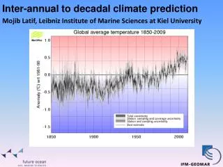
12. Approaches to Developing Probabilistic Seasonal Forecasts • Seasonal climate forecasting procedures usually start by examining historical climate records (Rainfall or Temperature), or a climatological database.  • The database should be long enough, complete and of good quality. • A standard 30-year period, such as 1961-90 or longer is applicable for most databases.

13. Cont.. • Various statistical analyses can then be carried out on the historical data and some relationships determined between potential predictors (e.g., ENSO and associated teleconnections) and the predictand (Rainfall or Temperature).   • The common predictor choices are usually lagged SST anomalies over the global oceans that are considered pertinent to the predictand.

14. Cont.. • The statistical associations between lagged SST indices and the climate variables can be found by performing simple correlation analysis between these variables.   • Once these have been established, what follows would be to develop either simple linear regression or multiple linear regression (deterministic) models relating the predictors with the predictands and use the model for prediction.

15. Cont.. • Several other potential predictors such as QBO, SOI and SST gradients among others can be included in the development of the regression model. • Stepwise regression technique (forward/backward) can be applied in selecting the best predictors that are to be included in the multiple linear regression equation.

16. Stepwise Regression analysis • Forward Selection: In this procedure, only the best potential predictors that improves the model the most, are examined individually and added into the model equation, starting with the one that explains the highest variance, etc. • Backward Elimination: The regression model starts with all potential predictors and at each step of model construction, the least important predictor is removed until only the best predictors remain. • A stopping criteria should be selected in both cases.

17. Use of the Linear Regression Fit • A linear regression model may depict positive or negative association between the predictors and the predictand. • Using this type of relationship, it is possible to make qualitative statements regarding the expected value of the predictand for the coming season(s) if knowledge of the seasonal lags of the predictor indices can be obtained in well in advance.

18. Goodness of fit measure • The goodness of “fit” of a linear regression model can be determined by examining the mean-squared error (MSE) in the ANOVA table output. This measure indicates the variability of the observed values around the forecast regression line. • A perfect linear relationship between the predictor and predictand gives an MSE of zero, while poor fits results in large values of MSE. • Another measure of the fit of a regression is the coefficient of determination (R2) which is, the squared value of the Pearson correlation coefficient between predictor and predictand.

19. Cont.. • Qualitatively, R2 can be interpreted as the proportion of the variance of the predictand that is described or accounted for by the regression. • For a perfect regression, the R2 = 1, while for R2 close to 0 indicates that very little of the variance is being explained by the regression line.

20. Examples of model fits

21. Examples cont..

22. Examples cont..

23. Verification of Forecast Skills • A number of quantities can be computed as a means of verifying forecast skills. These include: • Accuracy: Is a general term indicating the level of agreement between the Predicted value and the Observed value. The Error is the difference between the two values and the smaller the error the greater the accuracy

24. Cont.. • Skill: Thismeasures the accuracy of a given forecast relative to the accuracy of forecasts produced by some standard procedure. Skill scores provide a means of accounting for variations in accuracy that have nothing to do with the forecaster's ability to forecast.

25. Cont.. • Reliability or bias: This may be defined as the average agreement between the forecast value of an element and the observed value. A positive bias indicates that the forecast value exceeds the observed value on the average, while a negative bias corresponds to under forecasting the observed value on average. • Sharpness is the tendency to forecast extreme values

26. Computing Skill Scores Forecast Category Total J K L Total M N OT

27. Hit Score (HS) • Hit Score (HS): Number of times a correct category is forecasted

28. Post Agreement • Post agreement is the number of correct forecasts made divided by the number of forecasts for each category.These are: • A11/M, • A22/N, • A33/O

29. False Alarm Ratio (FAR) • False Alarm Ratio (FAR): The fraction of forecast events that failed to materialize • Best FAR=0; worst FAR=1 • For Above-Normal=(A21 + A31)/(M) • For Near-Normal=(A12 + A32)/(N) • For Below-Normal=(A13 + A23)/(O) • FAR = 1 – Post Agreement of the extreme event

30. Probability of Detection (POD) • This is the number of correct forecasts divided by the number observed in each category. It is a measure of the ability to correctly forecast a certain category, and is sometimes referred to as "Hit rate" especially when applied to severe weather verification. POD for the three different categories are: • A11/J, • A22/K, • A33/L

31. Bias • Bias: Comparison of the average forecast with the average observation • Bias > 1 : over-forecasting • Bias < 1 : under-forecasting • For Above-Normal=(M)/(J) • For Near-Normal=(N)/(K) • For Below-Normal=(O)/(L)

32. Heidke Skill Score This is given by where R = Total number of correct forecasts, T = Total number of forecasts, E = number expected to be correct based on chance, persistence, climatology

33. Zone 8 (Kerugoya) Forecasts Dry Normal Wet Total Percent Correct = 64% Dry Normal Wet OBS. Dry 3 0 0 3 Probability of Detection 100 50 50 Post Agreement 60 67 67 Normal 1 2 1 4 Wet 1 1 2 4 False Alarm (1st Order) 20 0 Hit Skill score (HSS) = 0.46 Total 5 3 3 11 Computational Example

34. Presenting Forecasts in terms of Probabilities • A standard format for presenting seasonal forecasts is by assigning percentage probabilities into what are known as terciles. • Terciles basically consist of three ranges of values that are used to represent three broad sectors of a normal probability distribution with equal chances of occurrence, climatologically, namely the lower, middle, and upper thirds of the expected distribution of values.

35. Cont.. • For example, a typical seasonal forecast may be presented as (45, 30, 25) and this can be interpreted as a 45% chance of seasonal total precipitation being in the upper (Wet) tercile, a 30% chance of it being in the middle or (Near normal) category, and a 25% chance that it may fall in the lowest third (Dry) category. • Seasonal forecasts presented in this way not only indicate the most likely outcome for the upcoming months or seasons, but also the distribution of possible outcomes. Such forecasts can take all the possible directions and can therefore never be wrong.

36. Example of tercile groupings

37. Example of a Seasonal ForecastGiven in terms of Probabilities

38. Making Decisions using Probabilities (Example) • Suppose that a farmer plants two main crops, Sorghum (S) or Maize (M). The yield response of Crop S with increase in rainfall is rather small but it does best if rainfall in the growing season is greater than 500 mm. During such seasons, the farmer can expect to earn about $120 per hectare. However, if rainfall is between 400 and 500 mm, the farmer can expect to earn up to about $100 per hectare. For seasons with rainfall between 250 and 400 mm, the crop yield will be smaller and the farmer can only earn about $60 per hectare from such yields.

39. Cont.. • On the other hand, Maize (Crop M), responds extremely well with increase in rainfall. For seasons with rainfall above 500mm, the farmer can earn about $200 per hectare. However, if rainfall is below 400 mm, there is a big chance of a complete crop failure and his investments in seed and fertilizer results in a $15 loss per hectare. The table below gives a summary of the various rainfall events and their corresponding probabilities estimated from a 10 year historic records. Also shown in the table are the likely earnings per hectare from S and from M crops.

40. 250 – 400 mm 400 – 500 mm More than 500 mm Historic Probability 30% 40% 30% Expected years in 10 3 4 3 Expected Crop S Earnings per Hectare ($) 60 100 120 Expected Crop M Earnings per Hectare ($) -15 120 200 Cont.. Total Rainfall in Growing Season (Source: IRI Exercise Website )

41. Cont.. • If the farmer plants crop S, then over a 10 year period he can expect to earn $60 in each of the 3 below normal seasons, $100 in each of 4 near normal seasons and $120 in the 3 above normal seasons. The total earning over a ten-year period is will then be $940, which averages to $94 earned per season per hectare planted. Similarly, if the farmer plants crop M, then over a 10 year period he can expect to lose the money invested in seed and fertilizer in 3 of the 10 years, but will earn $1080 in the other years. In the end, this strategy earns him an average of $103.50 per season per hectare planted.

42. Cont.. • It can be seen from this illustration that the average earnings over ten years will be somewhat higher with maize, but there are advantages and disadvantages to each crop. There is much less risk in planting sorghum, since one is assured of having something to harvest every year. On the other hand, many farmers would prefer planting maize due to ease of harvesting and post-harvest handling and good taste. Various strategies can be employed in balancing the risks and returns from these crops incase of change of the forecasts.