Download
1 / 28
280 likes | 381 Views
Explore the historical perspective and impact of seasonal climate prediction models at GFDL, emphasizing predictability, potential predictability, and practical applications. Discover how GFDL's climate prediction systems contribute to NOAA's long-lead forecasting products.

E N D
The Science of Seasonal Climate Forecasting Bill Stern GFDL/NOAA/Climate-Change-Variability-and-Predictionhttp://www.gfdl.noaa.gov/climate-change-variability-and-prediction http://www.gfdl.noaa.gov/bill-stern-gfdl-noaa Bill.Stern@noaa.gov 05 May 2011
Seasonal Climate Prediction at GFDL Motivation for Seasonal Prediction at GFDL: Contribute to NOAA long-lead prediction products Relevance to Society GFDL Historical Perspective Climate Prediction and General Circulation Models (GCMs) Predictability / Potential Predictability / “Practical” Potential Predictability Seasonal Prediction / Predictability Impact of SST anomalies. i.e., ENSO What happens when there is no El Nino or La Nina? A Simulated Seasonal Forecast Discussion Using available “End Stage” Internet Forecast Products
Multi-Decadal Scale Variability? Devils Lake, ND Lake Mead 2010 Nat Park Service USGS Goldenberg, et al., 2001
GFDL Historical Highlights (first 50 years) In 1955 the Weather Bureau created the General Circulation Research Section and appointed Joe Smagorinsky as its Director * 1955: Collaboration established between Princeton’s Institute for Advanced Study, the Weather Bureau, Air Force, and Navy to generate a computerized model of atmospheric circulation * 1967: First model estimate of the impact of carbon dioxide on global temperature * 1969: First model coupling the ocean and atmosphere completed (cited as a “Milestone in Scientific Computing” by Nature, 2006) * 1982: GFDL experimental NWP model physics transferred to NMC operational model * 1985: First diagnosis of weakening ocean circulation in a warming world * 1990: First simulation of Antarctic ozone hole; First GCM results used in IPCC. * 1991: First community global ocean model completed (MOM1) * 1995: GFDL Hurricane Prediction System made Operational at NWS/NMC * 2002: First realistic model study of impact of global warming on hurricane intensity * 2004: GFDL begins producing real-time seasonal forecasts * 2005: Development of CM2.0 and CM2.1 completed, two of the world’s leading climate models used in 2007 IPCC-AR4.
The Climate Prediction Problem Climate = set of statistics associated with many different states of the atmosphere/ocean (i.e., for an atmospheric/oceanic field - time and/or space and/or ensemble average, also PDF ).2 classes of climate prediction (Lorenz, 1975):1st kind = Initial value problem (i.e., future states of atmosphere-ocean depend on initial state.)2nd kind = forced boundary value problem with (How does a prescribed forcing, such as a doubling of CO2, affect a future climate state?) The Climate Predictability Problem Predictability for climate prediction of the 1st kind is limited due to rapid growth of errors in estimating the initial state (Lorenz, 1969). But predictability limit is extended for averaged fields relative to deterministic weather prediction because slower growing large errors between averaged fields is the limiting factor along with an ocean that varies on time-scales much longer than weather events. Ensembles provide a way to sample uncertainties/errors in initial states and models.
Ensembles and Averaging • Major Sources of Atmospheric Forecast Error Growth: • IC Uncertainty and Model Error • Errors Amplify due to the Chaotic Nature of the Atmospheric Equations resulting in Noise Dominating a Forecast • Noise can be reduced via Ensemble and Time (and Space) Averages • Furthermore, Ensembles can provide Probability Information Daily Monthly
General Circulation Model dV/dT = …. Fv dT/dT = …. FT dq/dT = …. Fq
GFDL Climate Prediction System - Overview Tier 1 Tier 2 Ocean Obs NCEP RA Obs SST Predicted SST ECDA CM2Ensembles Atmos IC AM2Ensembles AMIP Multi-year ensemble SST Forecasts Climate Forecast Products
Seasonal to Interannual (S/I) Prediction at GFDL GFDL Climate Prediction Systems: Tier 1 – Coupled Atmosphere-Ocean GCM (CM2): Hindcasts and now near real-time 10 member ensemble, 1 year predictions, 1979->, IC = Jan1, Feb1, …, Dec1 Tier 2 – Atmospheric GCM (AM2): Hindcasts from 1950 -> 2000 Real-time forecasts as part of the International Research Institute (IRI) multi-model ensemble - four 10 member ensembles (3 predicted SSTA + persisted SSTA), 7 month predictions, 2004 Aug ->, IC = Jan1, Feb1, …, Dec1 Where SSTA = sea surface temperature anomalies
Prediction and Predictability Metrics Anomaly Correlation Coefficients: time series (TCC); spatial patterns (ACC) Root Mean Square Anomaly Error (RMS) PDF: Ensemble Anomaly Probability Forecasts Ranked Probability Skill Scores (RPSS) Potential Predictability (perfect model scenario) Signal to Noise Ratio = S/N (>1) Signal (S) – Interannual Stnd. Deviation (ensemble mn) Noise (N) – Ensemble Stnd. Deviation (members)Ensemble spread or correlations (>0) within ensemble “Practical” Pot. Predictabilityallows for model/obs errors
Potential Predictability for 1991-2000 indicated via S/N ~1 or greater. AMIP (top left), Coupled (top right), Persisted SST (bot left),APCN Tier 2 (bot right)
Temperature changes associated with ENSO affect ocean ecosystems and global weather patterns, with far-reaching consequences for fisheries, agriculture, and natural disasters. Worldwide losses resulting from the 1997-98 El Niño are estimated at $32-$96 billion.
Ensemble Forecast Probability Distributions Tercile Forecasts - 3 category probability forecasts (above, normal, below), using historical GCM integrations to define range for forecast anomalies vs. historical record of observed anomalies. Calculate Ranked Probability Score (RPS) and then Ranked ProbabilitySkill Score (RPSS) following Wilks 1995 and Goddard et al., 2003, i.e., RPS = SUM(CPFm—CPOm)2, where m=1,3 and CP = cumulative probability of a category RPSS = 1- RPSfcst/RPSref , where ref = climatology
Skill Assessment for US 1997-98 Winter Season Precipitation Forecast Nov IC May IC
Coupled Model Cold Drift in Nino 3.4 Region (lat 5S-5N ave) – Jan IC
What Should We Do When There is no ENSO? • Why bother making a forecast since its going to be wrong anyway • Ask for help from friends and relatives • Go on extended vacations • Make a forecast with appropriate confidence information
North Atlantic Oscillation (NAO) This index measures the anomalies in sea level pressure between the Icelandic low pressure system and the Azores high pressure system in the North Atlantic Ocean. When the NAO is in its is positive phase (+NAO), the northeastern United States sees an increase in temperature and a decrease in snow days; the central US has increased precipitation, the North Sea has an increase in storms; and Norway along with Northern Europe has warmer temperatures and increased precipitation. When the NAO is in its negative phase (-NAO), the Tropical Atlantic and Gulf coast have increased number of strong hurricanes; NE US colder and snowier; northern Europe is drier and colder, and Turkey along with other Mediterranean countries has increased precipitation.
Atlantic Multi-Decadal Oscillation NOAA/AOML
Hi-Resolution Model development Simulated variability and predictability is likely a function of the model Developing improved models (higher resolution, improved physics, reduced bias) is crucial for studies of variability and predictability New global coupled models: CM2.4, CM2.5, CM2.6 26
Summary S/I Prediction • Results show significant “practical” potential predictability at leads of 5 months or more. “Perfect model” scenario extends potential predictability to at least 9 month lead. ENSO is key to extended S/I predictability. • Coupled model hindcasts show a significant cold drift across the east-sentral tropical Pacific (Nino 3.4) region which adversely affects longer lead prediction skill of T2m and precipitation in the Tropical Pacific. • Current research efforts to improve S/I prediction include: • Coupled assimilation scheme Investigating improvements to convective parameterization and prognostic clouds Higher resolution
Using Internet Forecast Tools/Products Seasonal Forecast Discussion http://www.cpc.ncep.noaa.gov/products/predictions/long_range/tools.html http://www.cpc.ncep.noaa.gov/products/predictions/90day/tools/briefing/index.html Other Real-Time Weather Links http://www.gfdl.noaa.gov/bill_sterns_weather_page