A Sub-quadratic Sequence Alignment Algorithm for Unrestricted Cost Matrices
A Sub-quadratic Sequence Alignment Algorithm for Unrestricted Cost Matrices. Maxime Crochemore Gad M. Landau Michal Ziv-Ukelson. Presentation. R89922024 蘇展弘 B86202049 葉恆青 R90725054 呂育恩 R90922001 張文亮 R90922091 游騰楷. Outline. Introduction and preliminaries. LZ-78. The basic concept.

A Sub-quadratic Sequence Alignment Algorithm for Unrestricted Cost Matrices
E N D
Presentation Transcript
A Sub-quadratic Sequence Alignment Algorithm for Unrestricted Cost Matrices Maxime Crochemore Gad M. Landau Michal Ziv-Ukelson
Presentation • R89922024 蘇展弘 • B86202049 葉恆青 • R90725054 呂育恩 • R90922001 張文亮 • R90922091 游騰楷
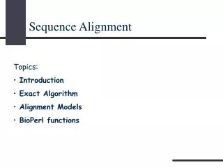
Outline • Introduction and preliminaries. • LZ-78. • The basic concept. • Global alignment. • Local alignment. • Proof for LZ-76. • Proof for SMAWK algorithm.
aacgacga 0 aacgacga g a 1 3 aacgacga c aacgacga 2 g 4 The number of distinct code word: aacgacga LZ-78 aacgacga aacgacga aacgacga aacgacga
c a t 3 1 0 4 5 2 3 1 2 0 4 g g a g c g Sample of LZ-78
Input border: I Diagonal prefix 0 0 0 0 1 1 1 1 2 2 2 2 3 3 3 3 4 4 4 4 a c g a a a a ac ac ac ac g g g g acg acg acg acg a a a a 1 1 1 1 c c c c a a c g 2 2 2 2 t t t t Top prefix 3 3 3 3 a a a a 3/2 3/4 3/4 a a c 4 4 4 4 cg cg cg cg g 5 5 5 5 ag ag ag ag 5/2 5/2 5/2 5/4 5/4 5/4 5/4 a a a a a Left prefix a c a a c c g g a c g a a a a g g g g Output border: O Basic Concept
OUT matrix 0 1 2 3 4 5 I0=1 1 0 -1 -2 -∞ -∞ I1=2 1 1 0 1 -1 -∞ Directly assign-∞ I2=3 1 3 3 4 2 0 DIST matrix I3=2 -12 0 0 2 0 0 0 1 2 3 4 5 0 1 2 3 4 5 I4=1 -13 -13 -1 1 0 0 I0=0 0 -1 -2 -3 △ △ I0=1 1 0 -1 -2 -∞ -∞ I5=3 -14 -14 -14 1 2 3 I1=0 -1 -1 -2 -1 -3 △ I1=2 1 1 0 1 -1 -∞ I2=0 -2 0 0 1 -1 -3 I2=3 1 3 3 4 2 0 I3=0 △ -2 -2 0 -2 -2 I3=2 -12 0 0 2 0 0 I4=0 △ △ -2 0 -1 -1 I4=1 -13 -13 -1 1 0 0 I5=0 △ △ △ -2 -1 0 I5=3 -14 -14 -14 1 2 3 OUT[i,j]=-(n+i+1) x k, Where k is the maximal absolute value in the penalty matrix. Oo O1 O2 O3 O4 O5 1 3 3 4 2 3 Basic ConceptI/O Propagation Across G DIST matrix
Def:A matrix M[ m x n ] is Monge if either condition 1 or 2 below holds for all a, b=0…m; c, d=0…n: 1. convex condition: 2. concave condition: Basic ConceptMonge Property DIST matrix Aggarwal and Park and Schmidt observed that DIST matrices are Monge arrays.
Def:A matrix M[ m x n ] is totally monotone if either condition 1 or 2 below holds for all a, b=0…m; c, d=0…n: 1. convex condition: 2. concave condition: Basic ConceptTatally Monotone An important property of Monge arrays is that of being totally monotone. Both DIST and OUT matrices are totally monotone by the concave condition. Aggarwal et al gave a recursive algorithm, nicknamed SMAWK, which can compute on O(n) time all row and column maxima of a n x n totally monotone matrix, by querying only O(n) elements of the array.
OUT matrix • concave monotonicity: 若左行的上面比下面小,則右行的上面也比下面小 • No new column maximum : • –(n + i + 1) * k • -
Maintaining Direct Access to DIST Columns • 目的: • 跑 SMAWK 時需要用到的OUT matrix 必須由 DIST和inplut來提供,並在Constant time內得到 OUT matrix 的每一格。但是Space 又不能超過。 • 作法: • 只存新產生的column,並維護一個data structure。
Time and Space Complexity • 作new column • 作DIST vector ( 即找出該DIST matrix所有的column) • 用SMAWK從這個DIST(加上input)算出 output maxima。 O ( t )
Total complexity O ( h n2 /log(n) ) h n /log ( n ) n
Sub-Quadratic Local Alignment Eric, Yu En Lu Information Management Dept. National Taiwan University
Sub-Quadratic Global Alignment • Exploits Redundancy among sequences resulted by Lempel-Ziv Compression (self-repeating) to obtain the sub-quadratic part
Sub-Quadratic Local Alignment • Requires additional knowledge of where a locally optimal string starts and ends • However, this algorithm is performed on a per-block basis, we have to compute additional information specific to a block • And then use it as the cue to the final score
Additional Information I F=max {MAX ti=0 {I[i]+E[i]}, C} E[k] C S[i]
Algorithm Body • Given: DISTG • Encoding • Compute values of E • Compute values of S • Compute values of C • Propagation • Compute values of O’ (modified from the O in global alignment) • Computing F • Seek Highest Score • Find the highest score F
Back-Tracking the Exact Path • Global Alignment • Local Alignment • Given the block with max F value • We seek its path through looking its max{lp, tp, dia} block recursively until the score 0
Time/Space Analysis • Encoding • E: max{E[i]lp, E[i]tp,DIST[I, lc]} O(t) • S: (all other can be copies, except..) Slr,lc = max{Slr-1,lc+W,Slr,lc-1+W,Slr-1,lc-1+W} O(t) • C: max{Clp, Ctp, S[lc]} O(1) • Propagation • O[i] = max{O[i], S[i]} O(t) • F=max {MAX ti=0 {I[i]+E[i]}, C} O(t) • Find F O(hn2/log2 n) • Total Complexity O(hn2/log n)
Further Improvements • Efficient alignment storage algorithm • Conditioned in “discrete weights” • Gives a minimal encoding to DIST (O(t) O(1) ) for G • Thus we obtain O(hn2/(log n)2) storage complexity in Global-Alignment problem • While time complexity is O(hn2/log n)
Now, we are going to have presentations onSMAWK & LZ-76 Thank you!
Reference : Lempel and Ziv,1976 “On the Complexity of Finite Sequences” The Maximum Numbers of Distinct Words Speaker : Emory Chang Date : 2002/1/31
0 1 1 2 1 0 4 3 What is a Distinct Word? • EX: (LZ78) A = {0,1} ,a = |A| = 2 S = 0101000 ,n = |S| = 7 0 0 • 1 • 0 1 • 0 0 • 0 we have four distinct words, and five steps to generate the sequence. 5
Notation • A : the set of alphabets • α : the number of alphabets • S : a sequence belong to A • n : the length of S • C(S) : production complexity of S • N : the maximum possible number of distinct words. n
The upper bound • Any sequential encoding procedure employs a parsing rule which a long string of data is broken down into words that are individually mapped into distinct words. • For every :
Special case(1/2) Let N denote the maximum possible number of distinct words. Clearly C(S) < N+1 (a possible exception of the last one) Consider the special case : The sequence is formed by all distinct words of length of one, two, …, k ex: S = 0 1 0 0 0 1 1 0 1 1 ex: S = 0 1 0 0 0 1 1 0 1 1 ex: S = 0 1 0 0 0 1 1 0 1 1 ex: S = 0 1 0 0 0 1 1 0 1 1 ex: S = 0 1 0 0 0 1 1 0 1 1 0 0 1 1 2 1 2 n = 1•2 + 2•2 1 1 0 0 3 4 5 6
Special case(2/2) The length of symbols at level i The number of nodes at level i
General Case Level k+1 The length of level k+1=k+1
Proof: Since We have from from Therefore
SMAWK A Linear Time Algorithm for the Maximum Problem on Wide Totally Monotone Matrices
Definition • Let A be an nm matrix with real entries. • Aj denote the jth column of A and Ai denote the ith row of A. • A[i1,…,ik;j1,…,jk] denote the submatrix of A. • Let j(i) be the smallest column index j such that A(i,j) equals to the maximum value in Ai.
j(i)=3 i=2
Definition • A nmmatrix A is monotone if for 1i1i2n, j(i1) j(i2). • A is totally monotone if every submatrix of A is monotone.
Another Definition • In the previous paper, the definition of totally monotone is: • A matrix M[0…m,0…n] is totally monotone is either condition 1 or 2 below holds for all a,b=0…n; c,d=0…m: • 1. Convex condition: M[a,c] M[b,c] M[a,d] M[b,d] for all a<b and c<d • 2. Concave condition: M[a,c] M[b,c] M[a,d] M[b,d] for all a<b and c<d • We use concave here.
Comparison • Now we want to compare these two definitions. • The definition in SMAWK’s paper is called Ds, The definition in this paper is called Dc (we need a transpose to match the row and column of these to definition).
Comparison(cont.) • To proof Dc Ds. • Dc holds on matrix A[0…n,0…m] • Let A’[i…i’,j…j’] be a submatrix of A, ii1i2i’, j1= j(i1), j2=j(i2) j1 j2. j1 a,b,c d e,f,g h So j1 j2 i1 i2
Comparison(cont.) • To proof Ds Dc • The matrix satisfies Ds but not Dc. • Dc is stronger.
Lemma 1 • We define an entry A[i,j] is dead if j j(i). • Lemma 1: • Let A be a totally monotone nm matrix and let 1 j1 j2 m. if A(r, j1)A(r,j2) then entries in {A(i, j2):1 i r} are dead. if A(r, j1)A(r,j2) then entries in {A(i, j1):r i n} are dead. j1 j2 i r i
REDUCE(A) • REDUCE(A) • C=A; k=1 • WhileC has more than n columns do • case • C(k,k) C(k,k+1) and k < n : k = k+1 • C(k,k) C(k,k+1) and k = n :Delete column Ck+1 • C(k,k) < C(k,k+1) :Delete column Ck; • if k>1 then k = k-1
REDUCE(A) <
REDUCE(A)
REDUCE(A) <