Factorial Survey Methods:
Factorial Survey Methods:. R. L. Brown, Ph.D. rlbrown3@wisc.edu. and the use of HLM, HOLIT, HULIT, and HLIT Models. http://www.son.wisc.edu/RDSU/library.html. RDSU. University of Wisconsin-Madison. Classic Reference.

Factorial Survey Methods:
E N D
Presentation Transcript
Factorial Survey Methods: R. L. Brown, Ph.D. rlbrown3@wisc.edu and the use of HLM, HOLIT, HULIT, and HLIT Models http://www.son.wisc.edu/RDSU/library.html RDSU University of Wisconsin-Madison
Classic Reference Rossi PH, Anderson AB. The factorial survey approach: an introduction. In Rossi PH, Nock SL, eds. Measuring social judgments: the factorial survey approach. Beverly Hills: Sage, 1982.
The use of vignettes in social science research has a long history, including applications in psychological research since the 1950s.
Basic Definition Factorial Survey Methods are a technique for applying experimental design to survey research.
FS Methodology • FS has been devised to help in the unravelling of complex choices • FS offer a better approximation to “real” cases than traditional survey questions • FS describe fictitious persons (families, organizations, etc.) whose relevant characteristics are described in sketches.
FS Methodology (continued) • FS are constructed using experimental design by systematically varying factors or characteristics. • FS may allow us to investigate hard to study issues due to simulation. • FS major limitation – reality?
Factorial Surveys typically use designs with repeated measures 2 factor designs
A1 A1 A1 A2 A2 A2 B1 B2 B3 B1 B2 B3 S1 4 1 2 5 6 3 S2 1 5 6 2 3 4 S3 3 4 1 6 2 5 Sk (A x B x S) Design Physician Trust A = Gender of physician, B = Race of physician
(A x B x S) Design Patient-level Si Vignette- level a1b1 a1b2 a1b3 a2b1 a2b2 a2b3 Repeated Measures Factorial Designs produce hierarchical or multilevel data.
Statistical Analysis Typically we want to study the relationships between variables both within and between levels. What’s the problem with using classic general linear modeling (GLM)?
Assumptions of the GLM • Cases are independently sampled from a normal distribution (Vignettes) • Vignettes are hierarchical not randomly sampled • The covariance between individual error terms is assumed to be zero • Since vignettes are judged by the same subject correlation between error terms is likely.
Responses may be categorical or unlimited continuous • Unlimited continuous = HLM (Hierarchical linear modeling) • Binary outcome = HLIT (Hierarchical Logit modeling) • Ordered categorical outcome = HOLIT (Hierarchical ordered logit modeling) • Unordered categorical outcome = HULIT (Hierarchical unordered logit modeling)
Example Brown, R. , Brown, R. L., Rounds, L., Castelaz, C., and Papasouliotis, O. Physicians' decisions to prescribe Benzodiazepines for nervousness and insomnia. Journal of General Internal Medicine, 1997, 12, 44-52. Brown, R., Brown, R. L., Edwards, J., and Nutz, J. Variation in a medical faculty's decisions to transfuse: Implications for modifying blood product utilization. Medical Care, 1992; 30(12), 1083-1096.
(A x B x C x D x E x S) Design A = Gender – 2 levels B = Race – 2 levels C = Psychiatric Diagnosis – 3 levels D = Patient Health Status – 2 levels E = Patient’s Reported Alcohol Use – 3 levels
Factor (C=3) Factor (D=2) Factor (E=3)
Male Female AA W AA W D1 D2 D3 HS1 HS2 HS1 HS2 HS1 HS2 AU1 AU2 AU3 AU1 AU2 AU3 AU1 AU2 AU3 Incomplete Factorial Design
The hierarchical logistic model poses two regression equations, one modeling the vignette effects within the respondents, and the other modeling respondent effects between respondents. First, for each respondent we model a separate within-respondent regression model: where pij = the prescribing probability for vignette i by physician j, xijp = the value of the vignette characteristics for vignette i and respondent j, bip = the regression coefficients within respondent j. for i = 1, 2, ..., k vignettes j = 1, 2, ..., n respondents, p = 0, 1, ..., p vignette variables.
Physician responses on the respondent level are subsequently predicted by the values of the corresponding vignette characteristics. Second, each of the regression coefficients from the above model may be represented as a between-respondents model: Where bim = the within-respondents regression coefficient for vignette characteristic m and physician respondent i, zri = the values of the respondent characteristics for physician respondent i, grm = the regression coefficient that describes the effects of respondent variables on the within-respondents relationships bim, uim = random errors.
The observed (0,1) prescribing response, at level 1, is yij ~ Bin(1, pij) with Binomial variance pij (1-pij). This assumption of binomial variation can be tests by fitting an ‘extra-binomial parameter’ s2e , so the vignette-level variance would be s2epij (1-pij). Estimates close to 1.00 indicate appropriateness of the binomial assumption.