Download
1 / 26
270 likes | 502 Views
General 2 k Factorial Designs. Used to explain the effects of k factors, each with two alternatives or levels 2 2 factorial designs are a special case Methods developed there extend to the more general case But many more possible interactions between pairs (and trios, etc.) of factors.

E N D
General 2k Factorial Designs • Used to explain the effects of k factors, each with two alternatives or levels • 22 factorial designs are a special case • Methods developed there extend to the more general case • But many more possible interactions between pairs (and trios, etc.) of factors
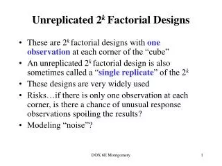
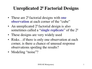
2k Factorial Designs With Replications • 2k factorial designs do not allow for estimation of experimental error • No experiment is ever repeated • But usually experimental error is present • And often it’s important • Handle the issue by replicating experiments • But which to replicate, and how often?
2kr Factorial Designs • Replicate each experiment r times • Allows quantification of experimental error • Again, easiest to first look at the case of only 2 factors
22r Factorial Designs • 2 factors, 2 levels each, with r replications at each of the four combinations • y = q0 + qAxA + qBxB + qABxAxB + e • Now we need to compute effects, estimate the errors, and allocate variation • We can also produce confidence intervals for effects and predicted responses
Computing Effects for 22r Factorial Experiments • We can use the sign table, as before • But instead of single observations, regress off the mean of the r observations • Compute errors for each replication using similar tabular method • Similar methods used for allocation of variance and calculating confidence intervals
Example of 22r Factorial Design With Replications • Same Time Warp system as before, but with 4 replications at each point (r=4) • No DLM, 8 nodes - 820, 822, 813, 809 • DLM, 8 nodes - 776, 798, 750, 755 • No DLM, 64 nodes - 217, 228, 215, 221 • DLM, 64 nodes - 197, 180, 220, 185
22r Factorial Example Analysis Matrix I A B AB y Mean 1 -1 -1 1 (820,822,813,809) 816 1 1 -1 -1 (217,228,215,221) 220.25 1 -1 1 -1 (776,798,750,755) 769.75 1 1 1 1 (197,180,220,185) 195.5 2001.5 -1170 -71 21.5 Total 500.4 -292.5 -17.75 5.4 Total/4 q0= 500.4 qA= -292.5 qB= -17.75 qAB= 5.4
N yi Estimation of Errors for 22r Factorial Example • Figure differences between predicted and observed values for each replication • Now calculate SSE
Allocating Variation • We can determine the percentage of variation due to each factor’s impact • Just like 2k designs without replication • But we can also isolate the variation due to experimental errors • Methods are similar to other regression techniques for allocating variation
Variation Allocation in Example • We’ve already figured SSE • We also need SST, SSA, SSB, and SSAB • Also, SST = SSA + SSB + SSAB + SSE • Use same formulae as before for SSA, SSB, and SSAB
Sums of Squares for Example • SST = SSY - SS0 = 1,377,009.75 • SSA = 1,368,900 • SSB = 5041 • SSAB = 462.25 • Percentage of variation for A is 99.4% • Percentage of variation for B is 0.4% • Percentage of variation for A/B interaction is 0.03% • And 0.2% (apx.) is due to experimental errors
Confidence Intervals For Effects • Computed effects are random variables • Thus, we would like to specify how confident we are that they are correct • Using the usual confidence interval methods • First, must figure Mean Square of Errors
Calculating Variances of Effects • Variance of all effects is the same - • So standard deviation is also the same • In calculations, use t- or z-value for 22(r-1) degrees of freedom
Calculating Confidence Intervals for Example • At 90% level, using the t-value for 12 degrees of freedom, 1.782 • And standard deviation of effects is 3.68 • Confidence intervals are qi-+(1.782)(3.68) • q0 - (493.8,506.9) • qA - (-299.1,-285.9) • qB - (-24.3,-11.2) • qAB - (-1.2,11.9)
Predicted Responses • We already have predicted all the means we can predict from this kind of model • We measured four, we can “predict” four • However, we can predict how close we would get to the sample mean if we ran m more experiments
N ym N N y ym Formula for Predicted Means • For m future experiments, the predicted mean is Where !
N y7 Example of Predicted Means • What would we predict as a confidence interval of the response for no dynamic load management at 8 nodes for 7 more tests? • 90% confidence interval is (811.6,820.4) • We’re 90% confident that the mean would be in this range
Visual Tests for Verifying Assumptions • What assumptions have we been making? • Model errors are statistically independent • Model errors are additive • Errors are normally distributed • Errors have constant standard deviation • Effects of errors are additive • Which boils down to independent, normally distributed observations with constant variance
Testing for Independent Errors • Compute residuals and make a scatter plot • Trends indicate a dependence of errors on factor levels • But if residuals order of magnitude below predicted response, trends can be ignored • Sometimes a good idea to plot residuals vs. experiments number
Testing for Normally Distributed Errors • As usual, do a quantile-quantile chart • Against the normal distribution • If it’s close to linear, this assumption is good
Assumption of Constant Variance • Checking homoscedasticity • Go back to the scatter plot and check for an even spread
Example Shows Residuals Are Function of Predictors • What to do about it? • Maybe apply a transform? • To determine if we should, plot standard deviation of errors vs. various transformations of the mean • Here, dynamic load management seems to introduce greater variance • Transforms not likely to help • Probably best not to describe with regression