Download
1 / 78
780 likes | 796 Views
Join the lecture series by Hirohito Yamada covering semiconductor photonics, electromagnetic wave interaction, optical amplification and more. The growth of internet traffic in Japan and the expanding application of optical communications devices will be explored. Learn about various photonic devices and their role in shaping the 21st century. Textbook titles include "Optical Communication Device Engineering" by Yasuo Yonezu and "Quantum Electronics" edited by Koichi Shimoda. Prepare for the future of optical communication technology!

E N D
Communications Devices Lecture from 5/8 Hirohito YAMADA
1. Schedule 5/8,5/15 Backbround of this lecture, Basic of semiconductor photonic devices5/22Matter-electromagnetic wave interaction based on semi-classical theory5/29Optical amplification and Laser6/26 Electromagnetic field quantization and quantum theory 7/3Optical transition in semiconductor, Photo diode, Laser diode7/10Optical amplifier, Optical modulator, Optical switch, Optical wavelength filter, and Optical multiplexer/demultiplexer About lecture 2. Textbook written in Japanese 米津 宏雄 著、光通信素子工学 - 発光・受光素子 -、工学図書 霜田 光一 編著、量子エレクトロニクス、裳華房 山田 実著、電子・情報工学講座15 光通信工学、培風館 伊藤弘昌 編著、フォトニクス基礎、朝倉書店 第5章 3. QuestionsE-mail: yamada@ecei.tohoku.ac.jp, or ECEI 2nd Bld. Room 203 4.Lecture note dounloadURL: http://www5a.biglobe.ne.jp/~babe
Growth of internet traffic in Japan Total download traffic in Japan was about 2.6T bps at the end of 2014 Daily average value Annual growth rate: 30% Total download traffic in Japan Total upload traffic in Japan 2004 2005 2006 2007 2008 2009 2010 2011 2012 2013 Cited from: H27年度版情報通信白書 year
Optical fiber submarine networks Cited from http://www1.alcatel-lucent.com/submarine/refs/index.htm
Power consumption forecast of network equipments Domestic internet traffic is increasing 40%/year If increasing trend continue, by 2024, power consumption of ICT equipments will exceed total power generation at 2007 Total power generation at 2007 Power consumption Total internet traffic (Tbps) Annual power consumption of network equipments (×1011Wh) Network traffic year http://www.aist-victories.org/jp/about/outline.html
Expanding applied area of optical communication Nowadays, application area of optical communications are spreading from rack-to-rack of server to universal-bass-interface of PCs Universal Bass interface (Light Peak) installed in SONYVAIO Z Backplane of a server (Orange color cables are optical fibers)
Various optical devices for use in optical networks 1.Passive optical device, Passive photonic device -Optical waveguide, optical fiber • Optical splitter -Optical directional coupler -Optical wavelength filter • Wavelength multiplexer/demultiplexer (MUX/DEMUX) • Light polarizer • Wave plate -Dispersion control device - Optical attenuator • Optical isolator - Optical circulator - Optical switch, Photonic switch -Photo detector, Photo diode (PD) : Treated in our lecture Photonic devices used for optical communications 2.Active optical device, Active photonic device -Light-emitting diode (LED) • Semiconductor laser, Laser diode (LD) • Optical amplifier 3.Other devices(Wavelength converter, Optical coherent receiver, etc.)
Various photonic devices used for applications other than optical communication • charge-coupled device (CCD) image sensor -CMOS image sensor -solar cell, photovoltaic cell • photo-multiplier -image pick-up tube • CRT: cathode-ray tube, Braun tube - liquid crystal display (LCD) - plasma display • organic light emitting display • various recording materials (CD, DVD, BLD, hologram, film, bar-code) • various lasers (gas laser, solid laser, liquid laser) - non-linear optical devices Photonic devices: supporting life of 21st century These devices collectively means “Photonic devices”
What is Photonic Device ? Manipulating electron charge Electronics voltage and current Manipulating wavefunction of electron Electron Tube, Diode, Tr, FET, LSI Tunnel effect devices Magnetic Recording Photo-electronics (Opt-electronics) Manipulating both spin and charge of electrons Display Spintronics CCD, CMOS sensor Manipulating photon and electron charge GMR HDD MRAM solar cell ? LD, LED Photo detector, PD Manipulating photon Unexplored Magnetics (Spinics) Photonics Opto-spinics Energy and number Laser magnet-optical disk HDD Optical disk Electromagnetic wave Magnetic tape Optical fiber Manipulating spin of materials amplitude and phase
105 T = 300K Si In0.53Ga0.47As 104 GaAs Optical absorption coefficient: α(cm-1) InP Ge 103 102 0.4 0.6 0.8 1.0 1.2 1.4 1.6 Wavelength: λ(μm) Properties required for semiconductor used as photonic devices Passive devices(Non light-emitting devices) ・ Transparent at operating wavelength Basis of semiconductor photonic devices ・ Small nonlinear optical effect (as distinct from nonlinear optical devices) ・ Better for small material dispersion ・ Small birefringence (polarization independence) Active devices(Light-emitting devices) ・ Moderately-opaque at operating wavelength ・ High radiant transition probability in case of light-emitting devices (Direct transition semiconductor ) ・ To be obtained pn-junction (To be realized current injection devices) Optical absorption coefficient of major semiconductor materials
Semiconductor and band structure According to Bloch theorem, wave function of an electrons in crystal is described as a quantum number called “wave number” This predicts existing dispersion relation between energy and wave number of electron. This relation is called energy band (structure) Band structure of semiconductors Electron In bulk Si, holes distribute at around the Γ point, on the other hand, electrons distribute at around the X point (Indirect transition semiconductors) Hole Band gap ~1.1eV Dispersion relation of electron energy in Si
Band structure of compound semiconductors Both electrons and holes distribute at around the Γ point (Direct transition semiconductors) Band structure of semiconductors Electron Electron Hole Hole GaAs InP
Band structure of Ge Ge which is group Ⅳ semiconductor is also indirect transition type semiconductor, but by adding tensile strain, it changes a direct transition-like band structure Band structure of semiconductors Recent year, Ge laser diode(RT, Pulse) was realized by current injection Band structure of Ge Conduction band Conduction band Indirect transition Direct transition 1.6% tensile strain Valence band Valence band
Material dispersion Values of dielectric constant (refractive index), magnetic permeability depend on frequency of electromagnetic wave interacting with the material Material equation Basis of semiconductor photonic devices Dielectric constant (refractive index) significantly changes at the resonance frequency of materials. In linear response, between real part and imaginary part of frequency response function holds Kramers-Kronig relation. Calc. Real part W. Sellmeier equation Photon energy (eV) Phenomenologically-derived equation of relation between wavelength and refractive index Calc. Imaginary part Here, λi = c/νi, c: light speed, νi: resonance frequency of material, Ai: Constant Photon energy (eV) Calculation of dielectric function ε of Si
Birefringence In anisotropic medium, dielectric constant (refractive index), magnetic permeability are tensor Basis of semiconductor photonic devices Optical axis Outgoing ray (Material equation) extraordinary ray Incident ray Crystal is optically anisotropic medium ordinary ray When light beam enter a crystal, it splits two beams (ordinary ray and extraordinary ray) In birefringence crystals, an incident direction where light beam does not split is called optical axis (correspond to c-axis of the crystal) Birefringence of calcite
Nonlinear optical effect Values of dielectric constant (refractive index), magnetic permeability depend on amplitude of electromagneticfield interacting with the material Material equation Basis of semiconductor photonic devices When strong electric field (light) applied to a material, nonlinear optical effects emerge. Wavelength conversion devices use this effects. When intensity of incident light is weak, linear polarization P which proportional to the electric field Eis induced. Linear polarization c: Electricsusceptibility When intensity of incident light become strong, electricsusceptibility become depended on the electric field E
Basis of semiconductor photonic devices Electron transition in direct transition type and indirect transition type semiconductors In case of indirect transition, phonon intervenes light emission or absorption Band structure of (a) GaAs and (b) Si
Excited state Nucleus Light absorption and emission in material All light come from atoms ! Sun light‥‥Nuclear fusion of hydrogen Light emission from materials Fluorescence of fireflies ‥‥Chemical reaction of organic materials Light Ground state Light from burning materials ‥‥ Chemical reaction of organic materials Excited state ν ΔE Light Electroluminescence from LED‥‥Electron transition in semiconductors Ground state ΔE = hν Why materials emit light? You have to learn about interaction mechanism of matter with electromagnetic field if you want to understand these phenomena In the field of Quantum electronics
v ω −e Electron m Proton r +e Rutherford atom model According to classical electromagnetics, Rutherford atom model is unstable. It predicts lifetime of atoms are order of 10-11sec. (See the final subject in my lecture note ElectromagneticsⅡ) Light emission from materials In order to solve this antinomy, Quantum mechanics was proposed N. Bohr proposed an atom modelwhich electrons exist as standing wave of matter-wave. The shape of the standing wave is defined by the quantum condition, and it is arrowed in several discreet states. When an electron transits from one steady state to other state, it emit / absorb photon which energy correspond to energy difference between the two states. (ΔE = hν) −e Proton +e Which process occur ? Light emission or absorption ? Bohr hydrogen atom model Why electrons make transition between the states ?
There are three methods describing interaction of matter with electromagnetic fields 1.Classical theory 2.Semi-classical theory Theory describing light absorption and emission Energy of electrons in semiconductor is quantized (Band structure), On the other hand, energy of electromagnetic field is treated by classical electromagnetics 3.Quantum theory Energy of electrons in semiconductor is quantized (Band structure), Electromagnetic field is also quantized (Field quantization) Three methods and their applicable phenomena Electromagnetic field Optical absorption Stimulated emission Spontaneous emission Matter Method Classical theory Classical Classical Possible Impossible Impossible Semi-classical theory Quantum Possible Possible Impossible Classical Quantum theory Quantum Quantum Possible Possible Possible
In order to understand interaction of matter with electromagnetic field, we need to describe electromagnetic field and to understand its fundamental characteristics Maxwell equations Description of electromagnetic field Electric fieldEand magnetic fieldBcan be also described as follows with electromagnetic potentialA(x, t) and ϕ(x, t) Therefore, Maxwell equations can be replaced to equations with Aand ϕas values of electromagnetic field, instead of EandB
Electromagnetic potentials can be described as follows with arbitrary scalar function χ(x, t). Description of electromagnetic field This function χ(x, t)is called a “gauge function”, and selecting these new electromagnetic potentialALand ϕL is called “gauge transformation”. Whenχ(x, t) was selected as ALand ϕL satisfying the following relation, the gauge is called “Lorenz gauge”. In this case, basic equations that describe electromagnetic phenomena is reduced to two simple equations regarding ALand ϕLas follows. These equations indicate that electromagnetic potentialALand ϕL caused by ie or epropagate as wave with light speed.
Other than Lorenz gauge, whenAwas selected as satisfying condition, the gauge is called “Coulomb gauge”. In this case, basic equations that describe electromagnetic phenomena is as follows Description of electromagnetic field In free space where both electric chargeρeand electric currentie do not exist, Therefore, Eand Bis derived from Awith the following relations By selecting Coulomb gauge,electromagnetic fields can be described by only vector potential A, because scalar potential ϕ is constant in whole space when electric charge dose not exist in the thinking space.
When single charged particle (electron) is in electromagnetic field, Hamiltonian of the particle is described as follows Interaction of charged particles with electromagnetic fields Here, p is the momentum operator, mis electron mass, Vis potential of electron, eis elementary charge, and A is vector potential. Hamiltonian H can be also written as, Here, H0 is an Unperturbed Hamiltonian which is for an electron in space without electromagnetic field, and Hintis an Interaction Hamiltonianwhich is originated by interaction between an electron and electromagnetic field. The last term in Hint is proportional to A2, and it reveals higher order effects (nonlinear optical effect). Here, we ignore it because the contribution is small.
Position of a charged particle is described as Polarization of electron cloud Momentum of a charged particle is described as E r Electrical-dipole approximation of the interaction Vector potential is described as Polarization of atom +e e+iωt E Electric field is e−iωt r −e Therefore, Electrical dipole Terms “ei2ωt”or“e−i2ωt” disappear when integrating for time Here, R = er, and it called electric dipole moment
Interaction Hamiltonian only include effect by electric field “RE” although the derived interaction equation for a charged particle include effects by both electric field (Coulomb force) and magnetic field (Lorentz force). The reason is that we assume the motion of a charged particle as which is vibration at a limited place. If we assume parallel motion for it, effect by magnetic field will be also included. Electrical-dipole approximation of the interaction In this way, when the interaction only depend on electric field, and the interaction can be described asRE, it is called electric dipole approximation. In some case, higher order polarization “multipolar” (such as electric quadrupole or electric octopole) occasionally emerge. Message to students Physical phenomena handled in engineering are usualy complicated. Therefore, it is impossible to construct a perfect theory incorporating all those physical phenomena.A good engineer is a person who can figure out what is essentially important among those phenomena, and use approximation appropriately although ignore the negligible physical phenomena, then build a simple theory. However, do not forget about what approximation was used.
In semiconductor, an electron and hole pair forms a electrical dipole Electrical dipole in semiconductor Conduction band Electron Electron −e Electrical dipole E Electrical dipole + +e Hole Hole Valence band Electrical dipole in semiconductor
Physical quantities involving many particles (electrons) such as electrical current are statistical average values for the particles. Furthermore, expected values for multiple measurements of a single event is needed statistical treatments. We discuss about statistical nature for many particles or multiple measurements. State for νth particle or νth measurement can be described as Quantum statistics and density matrix . Here, is an energy eigenstate for single particle. It is assumed to form complete space. Therefore, any can be formed bylinear combination of . does not required the suffix (ν). If operator for a physical quantity is assumed as A,expected value for νth particle is . Next, we develop an average of expected values for the group of particle (ensemble average).We assume the contribution from the νthe particle (probability for finding n th particle) as P(ν) , and normalize it.
Statistical average (ensemble average) of the expected value is described as Here, we rewrite as below Quantum statistics and density matrix Matrix ρhaving ρmn as its elements is called density matrix Using density matrix . is identity operator is summation of on-diagonal elements ofρA, that is Trace. , and
If we know the nature of the density matrixρ, we can obtain expected value including statistical nature, even we do not know the state of each particle in the group or the probability for finding n th particleP(ν). Then we direct equations for density matrix. Here, we rewrite the definition of matrix elements of density matrix as below Motion equation of density matrix Then, density matrix can be described as By differentiating both sides of this equation with respect to t, we can obtain Here, we assume probability for finding n th particleP(ν)is time independent.
From Schroedinger equation and its Hermitian conjugate , we obtain Motion equation of density matrix . This denotes time evolution of density matrix. Then we call it motion equation of density matrix or Quantum Liouville equation.
Assuming Hamiltonian operator of isolated electron systemis H0 and electric dipole moment isR, Hamiltonian operator interacting with electric fieldis denoted as Hint= −RE , and Hamiltonian operator for entire electron systemH is denoted as . Density matrix interacting with electric dipoles By substituting this in the motion equation of density matrix Here, it is assumed that the region where one electron is present is sufficiently smaller than the wavelength of the electromagnetic wave and the electric field can be regarded as constant within that range. In fact, the existence range of electrons bound to gas atoms is at most about several Å, and even at the electrons in the semiconductor, it is at most several tens of angstroms. On the other hand, since the wavelength of interacting light is several thousands Å, this assumption is valid.
Next, we derive equations for the matrix elements of the density matrix. Since there is no time dependency in energy intrinsic state, we can express as . Density matrix interacting with electric dipoles Therefore, we can write as . Here, the eigenstate used here is the eigenstate of the principal Hamiltonian H0.
Therefore, state takes the energy eigenvalueWn and there is orthogonality between the states, Density matrix interacting with electric dipoles . Here,ωmn is the angular frequency corresponding to the energy difference between the state m and state n.
First we consider interaction with the electromagnetic field in the two level system where there are only two possible energy levels of electrons. Upper(exited) state, Lower(bottom) state Wb Form = n = bin previous equation Interaction in two energy level system Wa Here, , ωaais also zero, and the diagonal matrix elementsRaa andRbb of the dipole moment R also become 0 in a general medium. Therefore As the same way, for m = n = a, . For m = b, n = aandm = a, n = b, We obtain . .
Here, ρbband ρaaare the electron distributions of the upper and lower levels, respectively. Therefore, . On the other hand, ρaband ρbarepresents the quantum correlation (quantum coherence) between the two states. These equations describe their temporal changes of them. The first equation shows the temporal change of electron distribution in the upper level, the second equation shows the temporal change of electron distribution in the lower level, and the third equation and the fourth equation describe the temporal change of the quantum coherence between these levels. Interaction in two energy level system These equations describe phenomena as light absorption and stimulated emission, but in actually there are the following phenomena not included in these equations. The electrons in the upper level transition to the lower level by stimulated emission and eventually no net emission occurs when the electron distribution is in the thermal equilibrium state. Therefore, in order to emit light continuously, it is necessary to pump the electrons in the lower level to the upper level. This is called pumping, and in semiconductor lasers, light emitting diodes and the like, pumping is performed by injecting a current into the pn junctions of the diodes.
The electrons in the upper level emit light at a certain rate even if no electromagnetic field is present, and transit to the lower level. This is called spontaneous emission. Spontaneous emission is caused by uncertainty when quantizing an electromagnetic field and can not be derived by dealing an electromagnetic field with classical theory (semi-classical theory). Interaction in two energy level system In deriving the density matrix so far, we did not consider collisions between particles or fluctuations of energy levels. However in actually, harmonic oscillations of dipoles are disturbed by collision between particle and the dipole oscillation is attenuated. This is called an electron relaxation effect (decoherence). Therefore, it is necessary to add such an effect phenomenologically.
Electron density of the upper level is increased (the lower level correspondingly decreases) by pumping rate: Λp, the electron lifetime time (also called longitudinal relaxation time) due to spontaneous emission: τs. Although the dipole oscillation decays by the collision between the particles etc., the lifetime (decoherence time) (also called the transverse relaxation time) : τd. Pumping and spontaneous emission are added to the diagonal elements of the density matrix and the lifetime of the dipole is introduced as a change in the off-diagonal elements. Therefore, as a phenomenologically corrected equations are described as follows. Interaction in two energy level system ρbb Wb spontaneous emission τs pumping Λp Wa ρaa
Next, find the solution of the differential equation, In the absence of an electric field, the above equation become a homogeneous equation Polarizability in 2 level system And the solution is Here, C is an arbitrary constant. On the other hand, under the presence of electric field, the solution can be described as with U(t). Substituting this into equation (4),
is obtained. Therefore, By integrating above equation with respect to time with electric field Polarizability in 2 level system (ρaa – ρbb)Rabis assumed to be constant within the integration time 0 ~ t Continue to next slide
Polarizability in 2 level system Here, considering the steady state of t >> τd
Furthermore, since ω≈ωba , the imaginary part of the denominator of the first term in {} is almost 0, but the imaginary part of the denominator of the second term is fairly large. Therefore, the second term in {} can be ignored. Then, Polarizability in 2 level system Similarly,ρbacan be obtained, but ρbais the complex conjugate of ρab, and ρba=ρ*ab. By the way, in classical electromagnetism, polarization P was Therefore, Here, Δt takes a time interval of about several times 1/ω
By the way, although the dipole efficiency R can be expressed as R = er, if this is used as a quantum mechanical operator and the electron density is Nt, polarization P is Polarizability in 2 level system Therefore, In this case, however, as described above, Raa = Rbb = 0 is considered.
The imaginary part of the polarizability χ represents the optical gain constant indicating the ratio of amplifying light when it is positive, and the optical attenuation coefficient in the case of negative. That is, the optical gain constant g is Optical amplification gain Unless it is a magnetic material, The total number of electrons present at levels b and a is Nt per unit volume. The electron density at level b is Nb, and the electron density at level a is Na. Since ρbb and ρaa indicate the ratio of the electron distribution, Therefore, optical gain is
In the thermal equilibrium without pumping, the electron distribution follows the Maxwell-Boltzmann distribution, Nb < Na, so the value of the optical gain constant g is negative. That is, light is absorbed by the medium. In photophysics, this is called basic absorption. On the other hand, when Nb > Nais realized by pumping, the gain constant becomes positive and the light is amplified and comes out. This is stimulated emission. The state of Nb > Na is called population inversion. Also, when Nb = Na, the medium is transparent. Population inversion Energy:E E Wb Wb Nb Nb Wa Wa Na Na Number of particles:N Number of particles:N thermal equilibrium(Nb <Na) population inversion(Nb >Na) Maxwell-Boltzmann distribution k: Boltzmann’s constant T: Temperature of material
When the optical electric field Ei is incident on the polarization P, Re χ Re χ ωba ω ω Here, when Im χ is negative, polarization oscillate with a delay of 0 to π/2 from the incident light Ei. Therefore, the photoelectric field Er emitted by the polarization is ωba Mechanism of optical amplification Im χ Im χ ω ω ωba ωba which delay π/2for polarization oscillation. Therefore, since the output optical electric field is synthesis of Ei and Er, the outgoing light is attenuated. (Right figure) ρbb < ρaa ρbb > ρaa On the other hand, when Im χ is positive, the polarization oscillates ahead 0 toπ/2forincident light Ei. The photoelectric field Er radiated by this polarization is delayed π/2 for polarization oscillation. Therefore, the output optical electric field is amplified. P 0 ~ π/2 0 ~ π/2 Ei Er Eout Ei P Eout Er attenuation amplification
Laser Positive feedback circuit Positive feedback circuitof lightwave Optical Amp. Amp. + Mirror Electric oscillator laser Light-matter Interaction The following three process are occurring at the same time electron E2 attenation amplification Light emission Incident light Outgoing light E1 twe-level system optical absorption stimulated emission spontaneous emission Laser is a light oscillator What is optical amplification medium?
Thermal equilibrium state Maxwell-Boltzmann distribution E n2: Number of atoms in the excited state k: Boltzmann constant T: Temperature of medium E2 stimulated emission E1 absorption absorption absorption P(E) In the thermal equilibrium state, the number of atoms in the excited level is smaller than the number of atoms in the ground level n1: Number of atoms in the ground state n1>n2 A: Einstein‘s A coefficient Probability of spontaneous emission= An2 B: Einstein‘s B coefficient Probability of absorption= Bn1 I Probability of stimulated emission= Bn2 I I: Intensity of incident light Net attenuation Bn1I > Bn2I In the thermal equilibrium state, the probability of absorption > the probability of stimulated emission, the incident light comes out with attenuation
Population inversion Population inversion T is negative(Negative temperature state) E n2: Number of atoms in the excited state E2 stimulated emission stimulated emission E1 Absorption P(E) stimulated emission A state in which the number of atoms in the excited level is larger than the number of atoms in the ground level is called a population inversion n1: Number of atoms in the ground state n1<n2 Net amplification Bn1I < Bn2I In the population inversion, the probability of stimulated emission> the probability of absorption, the incident light is amplified and comes out Laser is a device that creates population inversion by some method and amplifies light using stimulated emission of radiation
Laser Etymology of laser light amplification by stimulated emission of radiation maser microwave amplification by stimulated emission of radiation Type of laser A. Solid state lasers a. Lasers made of crystal Ruby(Cr3+: Al2O3) laser First oscillated laser in the world in 1960 Lasing by optical excitation λ = 694.3nm(red) Nd3+: YAG laserλ = 1064nm(near infrared) b. Glass laserDoped Nd into optical glass High power