Multi-resolution Resource Behavior Queries Using Wavelets
Explore the use of wavelets for fine-grain measurements in resource-appropriate multi-resolution views, addressing application-sensor tension and query models. Gain insights and promising results using a comprehensive approach.

Multi-resolution Resource Behavior Queries Using Wavelets
E N D
Presentation Transcript
Multi-resolution Resource Behavior Queries Using Wavelets Jason Skicewicz Peter A. Dinda Jennifer M. Schopf Northwestern University
The Tension Video App Sensor Fine-grain measurement … Resource-appropriate measurement Grid App Resource Signal (periodic sampling) Example: host load Course-grain measurement
Video Scheduling Video App Sensor Fine-grain measurements needed
Grid Scheduling Grid App Sensor Coarse-grain measurements sufficient
Interval Averages Application Sensor Average over interval Average over interval Ideal Result Adequate Result
Contributions / Outline • Application-sensor tension • Query model to address tension • Wavelets as basis for query model • Promising early results • Delay conundrum
Schematic Representation of Query Model Sensor Application ^ x x Lower bandwidth used Measurements at fs samples/second Desired rate at fq samples/second The desired rate signal is an estimate error = x – x ^
Sensor Application Query Stream + Error x t t Δ Δq
Sensor Application Query Average + CI (inow-N+1)D tnow=inowD x t t Application wants average over this interval Application gets average over this interval
Contributions / Outline • Application-sensor tension • Query model to address tension • Wavelets as basis for query model • Promising early results • Delay conundrum
Wavelets As Basis for Query Model • Natural time/frequency decomposition • Provides a multi-resolution view of a resource • Well known mathematical tool • Invented in the ’80s, hot in ‘90s and today • Linear complexity • Non-stationarity, other “normal” behaviors acceptable • Burrus, Gopinath, Gao, intro to wavelets and wavelet transforms: A primer • Analytic enabler • Prediction on different resolutions • Compression of measurement streams • … Queries over wavelet domain representation of signal
High Level View of a 4-level Wavelet Decomposition Sensor Level 0 Wavelet Transform Level 1 Wavelet Coefficients Level 2 Level 3 • Resource Signal is decomposed into levels • Samples at each level are at a different rate • Each level captures different frequency content • Corresponding inverse transform
4-level Wavelet DecompositionTime-frequency Localization Level Frequency 0 [0 fs/16] [fs/16 fs/8] 1 [fs/8 fs/4] 2 [fs/4fs/2] 3 x[n] [0 fs/2] Δ fs=1/Δ time
Example Decomposition of Host Load Lossless representation of resource signal
Computing Wavelet Coefficients • Streaming operation • Number of levels, M, chosen arbitrarily • Amortized work per sample: O(1) • O(n) for n samples • Block by block operation • Block of samples, n=2k • Levels, M = lg(n) + 1 • Circular convolution over block, O(n)
Application Proposed System Sensor Network Stream Interval Level 0 Level 0 Wavelet Transform Inverse Wavelet Transform Level L Level M-1 Level M Application receives levels based on its needs
Wavelet Compression Gains, 14 Levels Typical appropriate number of levels for host load, error < 20%
Contributions / Outline • Application-sensor tension • Query model to address tension • Wavelets as basis for query model • Promising early results • Delay conundrum
Load Traces • DEC Unix 5 second exponential average • 1 Hz sample rate • Traces collected in August 1997 • AXP0-PSC – Interactive machine with high load • AXP7-PSC – Batch machine • Sahara-CMU – Large-memory compute server • Themis-CMU – Desktop workstation • Windows 2000 percentage of CPU • 1Hz sample rate • Trace collected in May 2001 • Tlab-03-NU – Desktop, teaching lab machine
Testcases • Stream Queries • One million samples per trace • Interval Queries • 2, 8, 32, 128, 512, 2048, 8192 second intervals • 1000 randomized queries per interval length per trace
Performance Evaluation • Streaming queries metrics • Error variance • Error histograms • Error mean • Energy in error auto-covariance • Interval query metrics • Error variance • Error histograms • Error mean Error mean ~ 0 for all evaluations
Streaming Queries, Relative Error Variance Fewer than 1% of coefficients, error < 20%
Streaming Queries, Error Histogram at Level 6 Errors follow a near-Gaussian distribution
Interval Queries, Error Variance Error variance approaches zero as interval increases
Interval Queries, Error Histograms at Level 5 Distributions not always Gaussian
Contributions / Outline • Application-sensor tension • Query model to address tension • Wavelets as basis for query model • Promising early results • Delay conundrum
Block By Block System Delay M Levels Wavelet Transform Inverse Wavelet Transform ^ x[n] xr[n] … Block Block n samples in block n samples in block Sample Acquisitions Wavelet transform Inverse transform time Samples delayed by block size
Streaming System Delay, Example with Length 4 Wavelets (D4), 4 Levels Level 0 Length 22 Length 22 Level 1 Length 22 Length 22 xr[n-d] x[n] Level 2 Length 10 Delay K1 Length 10 Level 3 Length 4 Delay K2 Length 4 High levels delayed waiting for low frequency computations, output delayed by high order filter
Delay Conclusions • System implementation • Delay must be taken into account • Prediction may help reduce streaming delay • Application scheduling • Fine-grain apps more sensitive to delay • Coarse-grain apps less sensitive to delay • Suggestions? We are working on a solution!
Related Work • Database queries over wavelet coefficients • Shahabi, et al [SSDBM 2000] • Chakrabarti, et al [VLDB 2000] • Vitter, et al [CIKM ‘98, SIGMOD ‘99] • Network traffic analysis and modeling • Ribeiro, et al [IEEE INFOCOM 2000] • Riedi, et al [IEEE DSPCS ’99] • Feldman, et al [SIGCOMM ’98] • Wavelet theory • Daubechies [Ten Lectures on Wavelets ‘92, SIAM] • Mallat [IEEE Trans. on Pattern Analysis and Machine Intelligence, ’89]
Conclusions • Application-sensor tension • Query model to address tension • Wavelets as basis for query model • Promising early results • Delay conundrum
Future Work • Wavelets are an enabler of other techniques • Prediction over wavelet coefficients • Possibility of better results • Can reduce system delay • Further compression through processing • Adaptive decompositions based on resource • Looking at other resource streams • RPS implementation
Contact Information • Webpage • http://www.cs.northwestern.edu/~jskitz • Email address • jskitz@cs.northwestern.edu • Load traces and tools • http://www.cs.northwestern.edu/~pdinda/LoadTraces • Matlab scripts • Available by request (jskitz@cs.northwestern.edu)
Levels 0 1 2 3 f(Hz) f(Hz) fs/2 fs/16 fs/8 fs/4 fs/2 Frequency Information Vs. Rate Input Signal, x[n] Decomposition • Frequency information retained = fs/2 • Measurement rate, fs Q: Why is this true? A: The Nyquist Criterion- sampling theory
yl[n] Level 0 LPF x[n] 2 yh[n] Level 1 HPF 2 2 Downsampler y[n] c[k] ,for all k Wavelet Transform, 1 Stage LPF, HPF FIR filters x[n] y[n] h[n]
Level 0 Level 1 LPF LPF LPF Level M-1 Level M HPF HPF HPF Increasing Stages, Mallat’s Tree Algorithm x[n] Stages can be arbitrarily increased
Frequency Response • Filters must be even order for PR • Other special properties to retain PR • The filters are order N=8 (D8 wavelet) LPF HPF
Level 0 LPF 2 ^ xr[n] + Level 1 HPF 2 c[k] y[n] = 2 Reconstruction From the Wavelet Coefficients, 1 Stage Upsampler LPF, HPF time reversed filters, same response
Level 0 + Level 1 HPF HPF HPF LPF LPF LPF ^ + xr[n] Level M-1 + Level M Reconstruction From Multiple Stages, The Inverse Wavelet Transform Reconstructed signal is exactly the resource
Determined by accuracy constraints Determined by what levels are available Determined by the rate (fq) at which measurements are requested: Q: How are the number of levels determined? Answers:
Levels 0 1 2 3 f(Hz) fs/16 fs/8 fs/4 fs/2 Example, Choosing Levels Solution: L = 2: fq = fs / 6 M = 4 levels Equation Satisfied! Levels 0, 1 and 2 coefficients returned
Streaming Query Tradeoffs • Measurement rate, fqhigh • Lower error variance • Higher communication costs • Measurement rate, fq low • Higher error variance • Very low communication costs Wavelet approach yields accuracy at low rates
Interval length N long Less dynamic rate Tighter confidence intervals Interval length N short More dynamic rate Wider confidence intervals Rate, fq high Shorter interval length Tighter confidence intervals Rate, fq low Longer interval length Wider confidence intervals Interval Query Tradeoffs Confidence interval (c) provides flexibility
Streaming Queries, Energy in Auto-covariance Error becomes uncorrelated as levels added
Interval Queries, Error Mean (32 seconds) Error mean is zero at 8 levels, 3% of coefficients
Interval Queries, Error Mean (512 seconds ~ 8½ minutes) As interval increases, need fewer levels