Download
1 / 29
290 likes | 461 Views
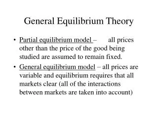
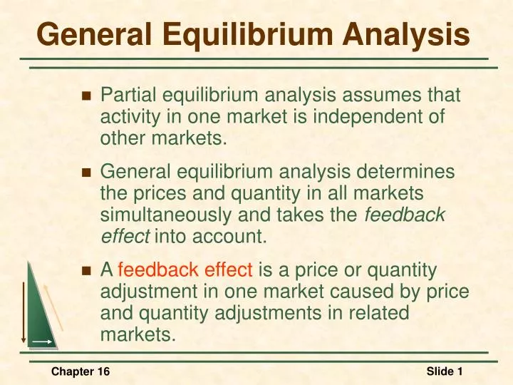
General Equilibrium Analysis. Partial equilibrium analysis assumes that activity in one market is independent of other markets. General equilibrium analysis determines the prices and quantity in all markets simultaneously and takes the feedback effect into account.

E N D
General Equilibrium Analysis • Partial equilibrium analysis assumes that activity in one market is independent of other markets. • General equilibrium analysis determines the prices and quantity in all markets simultaneously and takes the feedback effect into account. • A feedback effect is a price or quantity adjustment in one market caused by price and quantity adjustments in related markets. Chapter 16
Assume the government imposes a $1 tax on each movie ticket. General Equilibrium Analysis: Increase in movie ticket prices increases demand for videos. S*M SV SM $3.50 $6.35 $3.00 D’V $6.00 DM DV QV Q’V Q’M QM Two Interdependent Markets (Movie Tickets and Videocassette Rentals) Moving to General Equilibrium Price Price Number of Movie Tickets Number of Videos
The increase in the price of videos increases the demand for movies. The Feedback effects continue. SV SM $6.82 $6.75 $3.58 D*V $3.00 D*M $6.00 D’M DM DV QV Q*V Q”M Q*M QM Two Interdependent Markets (Movie Tickets and Videocassette Rentals) Moving to General Equilibrium Price Price S*M $3.50 $6.35 D’V Number of Movie Tickets Number of Videos Q’V Q’M
Efficiency in Exchange • Exchange increases efficiency until no one can be made better off without making someone else worse off (Pareto efficiency). • The Advantages of Trade • Trade between two parties is mutually beneficial. Chapter 16
Efficiency in Exchange • Assumptions • Two consumers (countries) • Two goods • Both people know each others preferences • Exchanging goods involves zero transaction costs • James & Karen have a total of 10 units of food and 6 units of clothing. Chapter 16
The Advantage of Trade James 7F, 1C -1F, +1C 6F, 2C Karen 3F, 5C +1F, -1C 4F, 4C Individual Initial Allocation Trade Final Allocation Karen’s MRS of food for clothing is 3. James’s MRS of food for clothing is 1/2. Karen and James are willing to trade: Karen trades 1C for 1F. When the MRS is not equal, there is gain from trade. The economically efficient allocation occurs when the MRS is equal. Chapter 16
Karen’s Food 4F 3F The initial allocation before trade is A: James has 7F and 1C & Karen has 3F and 5C. The allocation after trade is B: James has 6F and 2C & Karen has 4F and 4C. James’s Clothing Karen’s Clothing B 2C 4C +1C 1C 5C -1F A 6F 7F James’s Food Exchange in an Edgeworth Box 10F 0K 6C 6C 0J 10F
Karen’s Food A: UJ1 = UK1, but the MRS is not equal. All combinations in the shaded area are preferred to A. D James’s Clothing Karen’s Clothing C UJ3 B UJ2 A Gains from trade UJ1 UK3 UK2 UK1 James’s Food Efficiency in Exchange 10F 0K 6C Is B efficient? Hint: is the MRS equal at B? Is C efficient? and D? 6C 0J 10F Chapter 16
Any move outside the shaded area will make one person worse off (closer to their origin). B is a mutually beneficial trade -higher indifference curve for each person. Trade may be beneficial but not efficient. MRS is equal when indifference curves are tangent and the allocation is efficient. The Contract Curve: to find all possible efficient allocations of food and clothing between Karen and James, we look for all points of tangency between each of their indifference curves. Karen’s Food 10F 0K 6C D Karen’s Clothing James’s Clothing C UJ3 B A UJ2 6C 0J 10F UJ1 UK3 UK2 UK1 James’s Food Efficiency in Exchange Chapter 16
E, F, & G are Pareto efficient . If a change improves efficiency, everyone benefits. Contract Curve G F E The Contract Curve Karen’s Food 0K James’s Clothing Karen’s Clothing 0J James’s Food Chapter 16
Efficiency in Exchange • Application: The policy implication of Pareto efficiency when removing import quotas: 1) Remove quotas • Consumers gain • Some workers lose 2) Subsidies to the workers that cost less than the gain to consumers Chapter 16
Efficiency in Exchange • Equilibrium in a Competitive Market • Competitive markets have many actual or potential buyers and sellers, so if people do not like the terms of an exchange, they can look for another seller who offers better terms. • There are many Jameses and Karens. • They are price takers • Price of food and clothing = 1 (relative prices will determine trade) Chapter 16
Begin at A: Each James buys 2C and sells 2F Each James would move from Uj1 to Uj2, which is preferred (A to C). Price Line PP’ is the price line and shows possible combinations; slope is -1 P C Begin at A: Each Karen buys 2F and sells 2C. Each Karen would move from UK1 to UK2, which is preferred (A to C). UJ2 A UJ1 P’ UK2 UK1 Competitive Equilibrium Karen’s Food 10F 0K 6C At the prices chosen: Qd food (K) = Qs food (J) – competitive equilibrium. James’s Clothing Karen’s Clothing At the prices chosen: Qd clothing (James) = Qs clothing (Karen) – competitive equilibrium. 6C 0J 10F James’s Food
Competitive Equilibrium Karen’s Food 10F 0K 6C Price Line The MRSCF is equal to the ratio of the prices, or MRSJFC = PC/PF = MRSKFC. P James’s Clothing Karen’s Clothing C Point C shows that the allocation in a competitive equilibrium is economically efficient. If the ICs were not tangent, trade would occur. The competitive equilibrium Is achieved w/o intervention. UJ2 A UJ1 P’ UK2 UK1 6C 0J 10F James’s Food Chapter 16
Equity and Efficiency • In a competitive market, all mutually beneficial trades take place and the resulting equilibrium allocation of resources will be economically efficient (the first theorem of welfare economics) • Is an efficient allocation also an equitable allocation? • Economists and others disagree about how to define and quantify equity. Chapter 16
*Any point inside the frontier (H) is inefficient. *Combinations beyond the frontier (L) are not obtainable. OJ L E F *Movement from one combination to another (E to F) reduces one person’s utility. *All points on the frontier are efficient. H G OK Utility Possibilities Frontier Karen’s Utility Lets compare H to E&F. E&F are efficient: E&F make one person better off without making the other worse off. The Utility Possibilities Frontier indicates the level of satisfaction that each of two people achieve when they have traded to an efficient outcome on the contract curve. James’s Utility Chapter 16
Karen’s Utility OJ E F H G OK James’s Utility Equity and Efficiency • Is H equitable? • Assume the only choices are H & G • Is G more equitable? It depends on one’s perspective. • At G James’ total utility > Karen’s total utility • H may be more equitable because the distribution is more equal, therefore, an inefficient allocation may be more equitable. Chapter 16
Karen’s Utility OJ OK James’s Utility Equity and Efficiency • Equity & Perfect Comp.: A competitive equilibrium leads to a Pareto efficient outcome that may or may not be equitable. • Points on the frontier are Pareto efficient. • OJ & OK are perfect unequal distributions and Pareto efficient. • To achieve equity (more equal distribution) must the allocation be efficient? Chapter 16
Efficiency in Production • Assume • Fixed total supplies of two inputs; labor and capital • Produce two products; food and clothing • Many people own and sell inputs for income • Income is distributed between food and clothing Chapter 16
Efficiency in Production • Production in the Edgeworth Box • Each axis measures the quantity of an input • Horizontal: Labor, 50 hours • Vertical: Capital, 30 hours • Origins measure output • OF = Food • OC = Clothing Chapter 16
80F 25C D 10C 30C C B A 60F 50F Efficiency in Production Efficiency • A is inefficient • Shaded area is preferred to A • B and C are efficient • The production contract curve shows all combinations that are efficient Labor in clothing production 50L 40L 30L 20L 10L 0C 30K 20K 10K Capital in clothing production Capital in food production 10K 20K Each point measures inputs to the production A: 35L and 5K--Food B: 15L and 25K--Clothing Each isoquant shows input combinations for a given output Food: 50, 60, & 80 Clothing: 10, 25, & 30 30K 0F 10L 20L 30L 40L 50L Labor in Food Production
Efficiency in Production • Competitive Market Observations • The wage rate (w) and the price of capital (r) will be the same for all industries. • Minimize production cost • MPL/MPK = w/r • w/r = MRTSLK • MRTS = slope of the isoquant • Competitive equilibrium is on the production contract curve. • Competitive equilibrium is efficient. Chapter 16
Why is the production possibilities frontier downward sloping? Why is it concave? OF 60 B, C, & D are other possible combinations. B C A A is inefficient. ABC triangle is also inefficient due to labor market distortions. OF & OC are extremes. D OC 100 Efficiency in Production: Production Possibilities Frontier (derived from the contract curve) Clothing (units) Food (Units) Chapter 16
MRS = MRT 60 Production Possibilities Frontier Indifference Curve C 100 Output Efficiency Clothing (units) How do you find the MRS = MRT combination with many consumers who have different indifference curves? • Goods must be produced at minimum • cost and in combinations that match • people’s WTP. The efficient output • and Pareto efficient allocation occurs • where MRS = MRT Food (Units) Chapter 16
Efficiency in Production • Efficiency in Output Markets • Consumer’s Budget Allocation • Profit Maximizing Firm Chapter 16
Overview: The Efficiency of Competitive Markets • Conditions Required for Economic Efficiency • Efficiency in Exchange (for a competitive market) Chapter 16
Overview: The Efficiency of Competitive Markets • Conditions Required for Economic Efficiency • Efficiency in the Use of Inputs in Production (for a competitive market) Chapter 16
Overview: The Efficiency of Competitive Markets • Conditions Required for Economic Efficiency • Efficiency in the Output Market (in a competitive market) Chapter 16
Overview: The Efficiency of Competitive Markets • Conditions Required for Economic Efficiency • However, consumers maximize their satisfaction in competitive markets only if Chapter 16