General Equilibrium
General Equilibrium. Review: Efficiency condition (Consumption): MRS A xy = MRS B xy = P X /P Y 2. Efficiency condition (Production): MRTS X = MRTS Y = MP LX /MP KX = MP LY /MP KY 3. Efficiency condition (Product mix):

General Equilibrium
E N D
Presentation Transcript
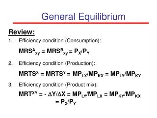
General Equilibrium Review: Efficiency condition (Consumption): MRSAxy = MRSBxy = PX/PY 2. Efficiency condition (Production): MRTSX = MRTSY =MPLX/MPKX = MPLY/MPKY 3. Efficiency condition (Product mix): MRTXY = - DY/DX = MPLY/MPLX = MPKY/MPKX = PX/PY
(1) Consumer Optimization Perfectly competitive markets: U= U(X,Y) subject to I =PX*X + PY*Y Optimization: where marginal utility equals price ratio Single consumer: Ux/PX = UY/PY Ux/UY = PX/PY = MRS
Slope = - UX/UY Equilibrium where UX/UY = PX/PY Consumer Optimization Y [I/PY] Indifference Curve:All possible combinations of good X and good Y which yield the same level of satisfaction Budget line:I =PX*X + PY*Y Y = [I/PY] – [PX/PY]X IC3 IC2 IC1 X
Consumer Optimization 0Sam QY A Edgeworth Box: At A: MRSPaul > MRSSam At B: MRSPaul = MRSSam = PX/PY B PX/PY 0paul QX
(2) Producer Optimization Perfectly competitive markets: single producer Maximize Qx = F(K,L) subject to C0 = wL + rK Thus: optimization when wage-rental ratio is equal to the slope of an isoquant: -DK/DL = MPL/MPK = w/r (Production Efficiency Condition)
Slope = - MPLX/MPKX Slope = - w/r Producer Optimization KX Isoquant:All possible combinations of capital and labour that could be used to produce a particular quantity of X Qx = MPLX*L + MPKX*K Isocost: C0 = wL + rK K = [C0/r] – [w/r]L Implies at equilibrium MPLX/MPKX = w/r [C0/r] X = 200 X = 150 X = 100 LX
E w/r Producer Optimization K 0Y 200 240 180 H A At H: MRTSX > MRTSY MPLX/MPKX > MPLY/MPKY X has too much capital, too little labour, Y has too much labour , too little capital >>> reallocation of capital & labour can increase output At E: MRTSX = MRTSY = w/r = MPLX/MPKX = MPLY/MPKY 100 C 80 D 150 240 200 0X L
(3) Product Mix Y Slope: - DY/DX or opportunity cost of producing 1 more unit of X in terms of Y forgone A Contract curve (Producer Optimization) and PPF (Production Possibility Frontier) 240 B 200 150 C - DY/DX 80 D 100 180 200 240 X
(3) Product Mix “Producing an efficient output mix involves balancing the subjective wants, or preferences (MRS of consumers) with the objective conditions of production”
(3) Product Mix Perfectly competitive markets: Two-good, two-factor model Qx = Fx(Kx,Lx) QY= FY(KY,LY) Factor market equilibrium (supply =demand) K = Kx + KY and L = Lx + LY Profit maximisation condition w = MPLX*PX r = MPKX*PX (1) w = MPLY*PY r = MPKY*PY (2) Rearrange (1) into (2): PX/PY = MPLY/MPLX = MPKY/MPKX But: MPLY = DY/DLY where : DLY = -DLX MPLX = DX/DLX Thus: MPLY/MPLX = -DY/DX = MRT PX/PY =
MPLY/MPLX = 2 (3) Product Mix Y Px/Py=5 A What is the incentive to shift from A to C under Px/Py = 5 ? 240 B 200 150 C - DY/DX 80 D 100 180 200 240 X
(2) Consumer optimisation: MRSA=MRSB=PX/PY (3) Product mix: MRTXY =PX/PY PX/PY (3) Product Mix (1) Producer optimisation: MRTSX=MRTSY (i.e. on contract curve) Y A 240 B 200 150 C 80 D 100 180 200 240 X
Production function Qx F(K0,L) Qx= F(K,L): Certain technology (F), which requires a combination of capital (K) and labour (L), can produce some quantity of good X (Qx). Assume: fixed capital (K0) >> Law of Diminishing Returns L MPLX L
Producer Optimization K A: MPL1> MPK1 K1 Marginal Rate of Technical Substitution MRTSA = MPL1/MPK1 > MPL2/MPK2 = MRTSB B: MPL2< MPK2 K2 L L1 L2
Producer Optimization K Isocost: C0 = wL + rK DC0 = wDL + rDK With DC0 = 0 wDL = - rDK w/r = -DK/DL (2) Optimization: where isoquant is tangent to isocost MRTS = MPL/MPK = w/r Isoquant: DQX = (MPL)DL + (MPK)DK With: DQX = 0 (MPL)DL = - (MPK)DK MPL/MPK = -DK/DL (1) w/r = MPL/MPK Kop L Lop