„Implementing Restricted Least Squares in Linear Models“
150 likes | 191 Views
Learn how to correctly interpret wage differentials using Restricted Least Squares (RLS) and how RLS is implemented in Stata for linear models. Explore the technical contributions and syntax of RLS, along with an illustrative example using the American Current Population Survey data. Enhance your regression analysis by understanding and applying RLS effectively.

„Implementing Restricted Least Squares in Linear Models“
E N D
Presentation Transcript
„Implementing Restricted Least Squaresin Linear Models“ Dr. John P. Haisken-DeNewjhaiskendenew@rwi-essen.de Haisken-DeNew / Stata 2006 Mannheim
1a. Background • Inter-Industry Wage Differentials- Why do secretaries in the steel industry make more money than otherwise observably identical secretaries in the services industry?- Calculating „wage differentials“: Wages in steel > services ?- Dummy Variables: 0 or 1 • Starting PointKrueger/Summers (1988) „Efficiency Wages and the Inter-Industry Wage Structure“, Econometrica, 56, p 259-93.- Would like to interpret differentials as deviations from a weighted average- Remove arbitrary selection of reference category - Excellent seminal paper, however technical problems …- Attempt to implement Restricted Least Squares (RLS) but.. - Incorrect standard errors: t-values systematically biased downward - Incorrect overall inference: Variation systematically biased downward Haisken-DeNew / Stata 2006 Mannheim
1b. Background • Technical Contribution (in Handout)Haisken-DeNew/Schmidt (1997) „Inter-Industry and Inter-Regional Differentials: Mechanics and Interpretation“, Review of Economics and Statistics, 79(3), p. 517-21.- How to implement Restricted Least Squares (RLS) correctly- How to implement RLS after any linear model (OLS, FE, RE…)- RLS was implemented in GAUSS, LIMDEP and Stata (crudely) • Now RLS is implemented in Stata in a flexible Ado <hds97.ado>- What does the syntax look like? Haisken-DeNew / Stata 2006 Mannheim
2a. RLS <hds97.ado> - One Dummy Set • Run a linear regressionreg/xtreg depvar indepvars • Standard Syntax (only ONE dummy set)hds97 indepvars [, options] options description refname( string ) a string containing the name of the "reference" categoryrealname( string ) a string containing a descriptive name for the set of dummy variablesweight( varname ) a string containing the name of the weighting variable Haisken-DeNew / Stata 2006 Mannheim
2b. RLS <hds97.ado> - Many Dummy Sets • Run a linear regressionreg/xtreg depvar x* Xvar_1 Zvar_1 Zvar_2 Dvar_* XXLvar_* • Advanced Syntax (MANY dummy variable sets) global hds97_1 Xvar_1 Xvar_ref descriptive_name_for_Xglobal hds97_2 Zvar_1 Zvar_2 Zvar_ref descriptive_name_for_Zglobal hds97_3 Dvar_* Dvar_ref descriptive_name_for_D ...global hds97_50 XXLvar_* XXLvar_ref descriptive_name_for_XXL (up to 50 globals/constraints can be set) Xvar_1 is a regressor used in regress or xtreg previously Xvar_ref is a text name for the reference category descriptive_name is a descriptive text name of the dummy set hds97 [, weight(wgt_var_name)] Haisken-DeNew / Stata 2006 Mannheim
2c. RLS <hds97.ado> • Output created by <hds97.ado>(A) Original Regression (OLS, RE, FE etc) repeated(B) Each Dummy Variable Group using RLS is calculated - From “k-1” Dummy Variables: “k” Coefficients reported(C) Weighted Standard Deviation (Sampling Corrected) of RLS Betas - Measure of overall variation (D) F-Tests of Joint Significance - Are the dummy variables as a group significant(E) Sample Shares of each Dummy - What were the sample shares used to create the weighted average - From the weighted average, the deviations are calculated (see B) Haisken-DeNew / Stata 2006 Mannheim
3. Illustrative Example (in Handout) • American Current Population Survey (CPS)- Use freely available January 2004 CPS sample- http://www.nber.org/morg/annual/morg04.dta • Run simple wage regression (age 18-65)- log hourly wages = f (age, gender, race, marital status, state) • Dummy Indicators- gender: male, female- race: white, black, other- marital status: married, divorced, separated, single- states: AK, AL… WY • Selecting arbitrary dummy variable as reference- Which one? Makes no difference in the calculation, just in interpretation • With RLS, interpret the dummy variables as deviations from a weighted average as opposed to an arbitrary reference category • If logged wages, then interpretation: %-point deviations from average • Use <hds97.ado> to implement RLS Haisken-DeNew / Stata 2006 Mannheim
3. Sample Regression Output (in Handout) • . regress lhw age genderm raceb raceo msmar msdiv mssep Source | SS df MS Number of obs = 8417-------------+------------------------------ F( 7, 8409) = 181.36 Model | 242.712792 7 34.673256 Prob > F = 0.0000 Residual | 1607.68867 8409 .191186665 R-squared = 0.1312-------------+------------------------------ Adj R-squared = 0.1304 Total | 1850.40146 8416 .219867093 Root MSE = .43725------------------------------------------------------------------------------ lhw | Coef. Std. Err. t P>|t| [95% Conf. Interval]-------------+---------------------------------------------------------------- age | .00861 .0004585 18.78 0.000 .0077112 .0095088 genderm | .1737988 .0095849 18.13 0.000 .1550101 .1925876 raceb | -.0730053 .0162526 -4.49 0.000 -.1048645 -.0411462 raceo | -.0131488 .0193254 -0.68 0.496 -.0510315 .0247338 msmar | .1365145 .0125807 10.85 0.000 .1118532 .1611758 msdiv | .1014927 .0180303 5.63 0.000 .0661489 .1368365 mssep | .0237369 .0341694 0.69 0.487 -.0432435 .0907174 _cons | 6.5783 .016593 396.45 0.000 6.545774 6.610826------------------------------------------------------------------------------ • . global hds97_1 genderm genderfgender. global hds97_2 raceb raceo racewrace. global hds97_3 msmar msdiv mssep mssglmarital. hds97 Name of reference description Haisken-DeNew / Stata 2006 Mannheim
3a. Gender (2-Way) Haisken-DeNew / Stata 2006 Mannheim
3b. Race (3-Way) Haisken-DeNew / Stata 2006 Mannheim
3c. Marital Status (4-Way) Haisken-DeNew / Stata 2006 Mannheim
3d. State of Residence (51-Way) Ref=Hi Haisken-DeNew / Stata 2006 Mannheim
3d. State of Residence (51-Way) Ref=Lo Haisken-DeNew / Stata 2006 Mannheim
3d. State of Residence (51-Way) Haisken-DeNew / Stata 2006 Mannheim
4. Conclusions • RLS: Interpretation of Dummy Variables- Even with a small dimension, RLS intuitive interpretation- Remove arbitrariness of reference category- Allow for importance weighting of each category • Easily Implemented with <hds97.ado>- Can be used afterregress or xtreg and coefficients calculated- Useful additional statistics calculated • Flexible use- Transform a single set of dummy variables- Transform up to 50 sets of dummy variables at once • Areas of Application- Wage Differentials by: Region, Industry, Occupation, Education, Marital Status, Race, etc… Haisken-DeNew / Stata 2006 Mannheim