Download
1 / 38
400 likes | 660 Views
II . Multiple Linear Regression (MLR). Least squares (LS) method is a tool for deriving approximate linear static models. However, LS will also be used in linear dynamic model parameter estimations.

E N D
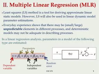
II. Multiple Linear Regression (MLR) • Least squares (LS) method is a tool for deriving approximate linear static models. However, LS will also be used in linear dynamic model parameter estimations. • Everyday experience shows that there may be (small/large) unpredictable elements in different processes, and deterministic models may not be adequate in describing processes. • In a linear regression analysis, parameters in a model of the following type are estimated: Parameters Random error Dependent variable Independent variables ChE 579 1 1
2.1. VariousResponse Surfaces β0is the y-intercept, i.e. E{y} at x1 = x2 = 0 ChE 579
2.2. Matrix Approach to MLR: How to find k = number of regressor variables n = number of observations n >> k L.S. estimate of βvector Residual vector ChE 579
Ex 1: Wine quality data. We would like to estimate the relation between quality (y), and concentration(x1), temperature (x2). ChE 579
2.3. Properties of L.S. Estimators • 1)Unbiased estimator: • 2)Consistent estimator: • i.e., as the sample size increases, interval estimates of estimators get narrower. • 3) Parameter estimates are independent only if the observations are independent If the columns are X are «close» to dependent, then det(XTX) will be close to zero and variance of the parameter estimates tends be very high. ChE 579
2.4. Significance of Regression Pressure (mmHg) vs. Concentration (g/m3) data Does β1 = 79.14 mean that there is a positive correlation between c and P? Please refer to your notes (1) Repeat the experiment with a larger number of samples to check the significance of β1. Not necessarily, because the C.I. of β (-316.4 < β< 474.6) contains 0! ChE 579
2.5. Model Adequacy Checking I) R2 value Ex 2: P vs. T data β1 β0 Model 1: β2 Model 2: β0 β1 Which model is better? ChE 579
Perfect fitting Total sum of squares Sum of squares of error Please refer to your notes (2) Model 1: Model 2: More satisfactory model ChE 579
II) Residual Analysis Model 1: Ex 2 contd: P vs. T data Residuals show a trend w.r.t. T! Model 2: Residuals do not show a trend w.r.t. T For a reliable model, residuals should be structureless! ChE 579
Model 1: Model 2: Normal probability plot For a reliable model, residuals should be normally (Gaussian) distributed! ChE 579
Ex 3: Price of oil vs. interest of treasury notes Step I. Plot data points >> scatter(x, y) >> xlabel('% interest') >> ylabel('$ oil') Step II. Determine a preliminary model type/order , perform regression. There seems to be a linear relation between % interest and $ oil. >> X = [ones(12, 1) x]; % construct the X matrix >> [b, bint, r, rint, mystats] = regress(y, X, .05); % fit y = Xb + model ChE 579
Step III. Check whether the full regression is significant. Check the p-value of the F-test. Check the R2 value. >> mystats >> 0.9397 155.8345 0.0000 5.0481 • P-value is pratically zero, meaning that the regression model is significant, as visual inspection also (obviously) shows. • R2 value is above 0.9, showing very good fit. Actually too good to be true! In real life, models with R2 >~0.7-0.8 are regarded as very good fits. Step IV. Plot the regression line (curve), and show the parameter estimates with their (1-)% confidence intervals. >> b b = -15.4750 3.7142 >> bint bint = -22.3400 -8.6100 3.0512 4.3771 ChE 579
>>scatter(x,y) >>refcurve(flipud(b)) Step V. Analyze the residuals: are they normally distributed and structureless? >> subplot(3, 1, 1) >> normplot(r) >> subplot(3, 1, 2) >> stem(x, r), xlabel('% interest (x)'), ylabel('residual') >> subplot(3, 1, 3) >> ypred = X*b; >> stem(ypred, r), xlabel(‘$ oil (yhat)'),ylabel('residual') Residuals are structureless, regression model is satifactory. ChE 579
III) Detection and Removal of Outliers • Inspect the outliers. • If you can detect a structural problem with these data points, remove the outliers, repeat the LS analysis. Report both analyses. • If you cannot detect any problem, leave the outliers. Out of confidence limits! Studentized Residual: ri ChE 579
IV) Model Robustness Ex 2 contd: P vs. T data Model 5: Model 6: Model 1: Model 2: Model 3: Model 4: Is the 6th order polynomial best model? ChE 579
As you increase the order of the model polynomial, R2 value will get closer to unity. When to stop? Why bother about the polynomial order? What is wrong with taking the highest order polynomial? Because a(n) (unnecessarily) high order polynomial would not be ROBUST. Model would explain the training set well, but would be poor in explaining the test set. Higher order terms would model the noise. ChE 579
How to choose a robust model? Cross-validation: Omit the ith observation, find for the model. Call these coefficients . Using , predict yi. Call this prediction . Find PRESS as follows: For the previous question: 4) Find the PRESS (Prediction error sum of squares) values for different models. Choose the model with the smallest PRESS. 2nd order polynomial has the smallest PRESS residuals. ChE 579
How does cross-validation work? True Model: • As expected, increasing the order of the polynomial decreases the SSE. • Actually, adding a cubic term would result in a curve passing exactly through the four data points (R2 = 1). • Those observations show that decreasing SSE should not be the justification for increasing the polynomial order unnecessarily. ChE 579
Omit sample #1, construct both models using the rest of the data points. Estimate y1, using the new model and x1. Omit sample #2, construct both models using the rest of the data points. Estimate y2, using the new model and x2. PRESS (linear model) = 0.64052+ (-0.0627)2+(-0.6981)2+1.13472 = 2.1891 PRESS (quadratic model) = 4.8843 • Continue this precedure for all data point. • Prediction errors are smaller in the linear model. • Linear model changes less (more robust) compared to quadratic model. ChE 579
Ex 4:Hollywood movies data (all data in million $) x1 Step I. Plot data points >> gplotmatrix(x, [x y]) x2 • Linear relation between x1 and y, x2 and y. Relation between x3 and y? • Columns of x are moderately correlated. x3 y ChE 579 x3 x2 x1
Step II. Determine a preliminary model type/order , perform regression. >> model1 = regstats(y, x, [0 0 0; 1 0 0; 0 1 0]); % no need to construct X matrix Step III. Check whether the full regression is significant. Check the p-value of the F-test. Check the R2 and R2adj values. >> model1.rsquare 0.9537 >> model1.adjrsquare 0.9405 >> sum((model1.r + model1.dffit).^2) 1359.2 >> model1.fstat sse: 475.3703 dfe: 7 dfr: 2 ssr: 9.7983e+003 f: 72.1417 pval: 2.1309e-005 Step IV. Show the parameter estimates with their p-values of their t-test scores. >> model1.tstat.beta 11.8482 4.2282 7.4361 >> model1.tstat.pval 0.1233 0.0080 0.0045 >> model1.tstat beta: [3x1 double] se: [3x1 double] t: [3x1 double] pval: [3x1 double] dfe: 7 ChE 579
Step V. Analyze the residuals. >> normplot(model1.r) >> stem(model1.studres) >> gplotmatrix([x(:, 1:2) model1.yhat], model1.r) Outlier! ChE 579
Step VI. Repeat the analysis omitting the outlier (sample #8) >> model1.tstat.pval 0.0040 0.0027 0.0000 >> model1.rsquare 0.9934 >> model1.adjrsquare 0.9912 >> sum((model1.r +model1.dffit).^2) 135.7043 Step VII. Repeat the analysis including x3 PRESS values of the second model is smaller! >> model2 = regstats(y, x, [0 0 0; 1 0 0; 0 1 0; 0 0 1]); >> model2.tstat.pval 0.0105 0.0030 0.0000 0.1387 >> model2.rsquare 0.9959 >> model2.adjrsquare 0.9935 >> sum((model2.r +model2.dffit).^2) 123.6470 ChE 579
Step VIII.Analyze the residuals again. • No outliers. • Residuals deviate from normality, but tolarable for small number of samples. • No trend of residuals detected. ChE 579
Step IX.Present the resulting model with the p-value of the F-test, R2 value, point estimates and 95% confidence intervals of parameters. >> [b, bint, r, rint, stats] = regress(y, [ones(size(x, 1), 1) x], .05); 95% CIs of Parameters Only if the units of regressors are identical!!! Step X. Interpret the model Sign of the ith parameter gives the direction of the partial effect of the ithregressor on the dependent variable. Magnitude of the ith parameter gives the size of the partial effect of the ithregressor on the dependent variable. • All three regressors have a positive effect on box office of the movie. Hence, high promotion-production costs and box sales tend to increase the box office success of a movie (makes sense!). • Effect of promotion costs is much higher than that of production costs, which, in turn, is higher than that of book sales on box office. Hence, key to box office success of a movie seems to be promotion (makes even more sense!) ChE 579
2.6. Selection of Variables and Model Building • The problem consists of selecting an appropriate SUBSET of regressors from all the regressors. The most common methods are: • All possible regressions, • Backward elemination, • Stepwise regression, etc. • In all possible regressions, if there are K regressors, there are 2K possible regression equations. • Ex. If K= 2 (x1 and x2), then the possible regression models are: • y = 0 • y = 0 + 1x1 • y = 0 + 2x2 • y = 0 + 1x1 + 2x2 • Examine all possible regression models using a criterion such as adjusted R2 and/or PRESS residuals, and find the best model. • For high values of K, constructing all 2K models is not feasible. • In backward elimination, start with all K regressors included. Then, delete the regressors with the smallest insignificant t-values one by one, until no further regressor can be deleted at the given criteria of significance (see the next section). ChE 579
Stepwise Regression • A sequence of regression models is constructed by adding or removing variables at each step. Criterion in addition/removal of variables is the t-test (or partial F-test): • Choose in and out: Limiting -values to accept addition (p <in) and removal (p > out) of variables into/from the model, respectively. One may use in = 0.10 and out = 0.15 for decreasing type-II error. It is useful to experiment with different in and out values. • Form a one-variable model using the regressor variable that has the highest correlation with the response variable. Suppose x1 is selected. • The remaining K-1 variables are examined for their t-values. Given x1 in the model, • Construct y = 0 + 1x1 + 2x2 , and compute t2,then • Construct y = 0 + 1x1 + 3x3 , and compute t3, then • Construct y = 0 + 1x1 + jxj , and compute tj. • The regressor with the highest t-value and satisfying p <in is accepted into the model. • Repeat the above procedure till there is no regressor left with p <in. Also, at any step if p > out for any of the previously added variables, then remove it. • Unlike all possible regressions, stepwise regression gives a local maximum. • Be careful, stepwise regression is prone to overfitting data! ChE 579
Ex 5:Stepwise regression example 1: Purity vs. concentration >> load lecture_stepwise_reg_ex1 >> gplotmatrix(X, [X Y]) >> corr([X Y]) 1.0000 0.8780 0.3021 0.0569 0.7750 0.8780 1.0000 0.2308 0.0511 0.6815 0.3021 0.2308 1.0000 0.0314 0.7863 0.0569 0.0511 0.0314 1.0000 0.0751 0.7750 0.6815 0.7863 0.0751 1.0000 • The last row in the graph matrix shows the high correlation between x3-y and x1-y: X1Y = 0.775 and X3Y = 0.787. • Regressor x2 has also high correlation with y (X2Y = 0.682), but it is also highly correlaled with x1(X1X2 = 0.878). This hints the possibility that using x1 and x2 simultaneously in the regression model may be redundant (overfitting). • Regressor x3 is moderately correlated with the other regressors, but highly correlated with y, showing that x3 is likely to be present in the regression model. • Regressor x4 is negligibly correlated with other regressors, but its correlation with y is also very low (0.075 - see also the last row-last column in the graph matrix). ChE 579
>> stepwise(X, Y) Blue lines denote the regressors included in the model Point estimates and confidence intervals of ’s. • Regressors are added in the order of x3 and x1. • P-value of is x2 given x3 and x1 are already in the model is 0.07 > 0.05 (the default value of in). • Hence, x2 is NOT added to the model, and the resulting regression model is • y = 0 + 1x1 + 3x3 ChE 579
Start at another inital model structure, e.g. y = 0 + 4x4 , to see if the same model is reached. At the end, it is seen that the same model is reached. >> stepwise(X, Y, logical([0 0 0 1])) ChE 579
Increase the in and out values to decrease type-II error, i.e. not to neglect any valuable information in X matrix that can be used in modeling y. >> stepwise(X, Y, [], .10, .15) This time, x2 is also included in the model: y = 0 + 1x1 + 2x2 + 3x3 ChE 579
The picture emerged so far is a competition between two models! Compare the adjusted R2 values and PRESS residuals of both models. >> model1 = regstats(Y, X, [0 0 0 0; 1 0 0 0; 0 0 1 0]); >> model2 = regstats(Y, X, [0 0 0 0; 1 0 0 0; 0 1 0 0; 0 0 1 0]); Although the improvement of R2 and adjusted R2 values on the inclusion of x2 is small, decrease of PRESS residuals implies that the additional regressor in model2 may be worthy of its predictive power. Next, we check the existence of outliers, using studentized residuals. >> stem(model2. studres) All studentized residuals lie in ~(-3, 3). ChE 579
Next, we check the distribution of residuals. >> normplot(model2. r) Distribution of residuals is close to normal. Last, we check the structure of residuals w.r.t. X and predicted values of y. • Residuals do not seem to have a trend with respect to regressors. • Note that residual vs. x4 is also plotted, though x4 is not included in the model. If a trend were detected in residual vs. x4 plot, then this would mean that x4 should be included in the model. • Nevertheless, there seems to be trend in residuals vs. predicted y values plot. Including higher order terms of regressors in the model may eliminate this trend! ChE 579
Hence, a suboptimal model is obtained as: >> model2.beta -8.9085 0.5799 0.0965 0.0624 >> CI = tinv(.975, 100-3-1)*model2.tstat.se 1.7092 0.1236 0.1052 0.0054 >> [model2.beta-CI , model2.beta+CI] -10.6177 -7.1993 0.4563 0.7034 -0.0087 0.2018 0.0570 0.0679 95% CI’s Conclusion: Quality variable is affected by three concentration measurements (x1, x2, x3) all in a positively correlated fashion. Though 3 has the lowest value, it does not mean x3 has the smallest effect on y, since range of is x3 is one order of magnitude higher than those of x1 and x2 (i.e. draw the boxplots x1, x2, x3). ChE 579
2.7. Effect of Dependeny Between Regressor Variables on Parameter Estimates • Is it advantegous to use multiple variables (regressors) for modeling the response of a quality variable? • Yes, but only if the variables are independent from each other. However, in real processes, measurements of different variables are often highly correlated. • For instance, temperature measurements along a plug flow reactor are highly dependent to each other. If we use all the temperature measurements to model the exit concentration, it is likely that we are going to be using a higher number of regressor variables than necessary. • This results in a unnecessarily high number of dependent parameters, which makes the model difficult to interpret and use, and larger confidence intervals for parameters, decreasing the precision of the model. ChE 579
Ex 4: Real Model: Only T1 is used to model c. Three highly dependent measurents, T1 , T2, T3 are used to model c. Due to the dependence of T1 and T2, data does not lie on a plane, but lie on a line. • Real parameter values lie within the confidence limits. • Confidence limits are remarkably wide (and contain 0). R2 = 0.845 PRESS = 17.48 R2 = 0.847 PRESS = 18.94 • Real parameter values lie within the confidence limits. • Confidence limits are narrow. • Improvement in R2 is insignificant. • PRESS is larger. ChE 579
So what should be done to model a high dimensional system? • Select and measure independent regressor variables. However, this is rarely possible (or practical) for actual processes. • Use stepwise regression or all possible regressions methods to select the regressor variables, which actually explain the output variable. The shortcomings of this method are: • For a large number of variables, it may be time consuming to decrease the number of variables in the model to a manangable number. • The regressor variables, which are left out of the model, may still have (individually small, but collectively significant) explanation power of the output variable. • Multivariable dimension reduction techniques, such as Principal Components Analysis (PCA), and Projection to Latent Structures (or Partial Least Squares, PLS) may be used to include all the measurements in the model, but define new independent variables (principal components, or latent vectors) which explain the given data set in largest amount. ChE 579