Download
1 / 26
260 likes | 401 Views
This presentation was held within the project ADVANCE, which has received funding from the European Union’s Seventh Framework Programme for research, technological development and demonstration under the grant agreement no 308329.

E N D
This presentation was held within the project ADVANCE, which has received funding from the European Union’s Seventh Framework Programme for research, technological development and demonstration under the grant agreement no 308329. Modeling Technological and Behavioral Response to Transport Policies Mark Jaccard (and Jonn Axsen) Simon Fraser University Vancouver Workshop on Transport Modeling in IAMs IIASA, Austria
Key points I explain how we pursue greater technological and behavioral detail in a nationally-focused hybrid simulation model. (The work of many researchers over at least a decade.) I explain the empirical research to estimate key parameters and their potential dynamism over time. I also explain how this work can inform less detailed, global models. Why? Policies are often technology and fuel specific (regs, subsidies), and they may try to change the decision context (urban form, transit and other non-vehicle options, road pricing). Why not? Potentially overwhelming in terms of data and research needs and model complexity.
Hybrid models (e.g., NEMS, CIMS) Combine the useful attributes of bottom-up (technological explicitness) and top-down (behavioral realism, equilibrium feedbacks) Jaccard, 2009, “Combining top-down and bottom-up in energy-economy models” in Evans and Hunt (ed.), International Handbook on the Economics of Energy.
CIMS: technology vintage model • Retire oldest stock (age-dependant) • Forecast demand – initial exogenous forecast adjusted by endogenous energy price and macroeconomic feedbacks (including service demand for personal mobility and freight) • Retrofit existing stock if economic (technology choice algorithm) • Calculate new stock purchase (demand minus existing stock) • Acquire new stock as needed (technology choice algorithm)
Personal Transportation Inter-city (Land) Urban Inter-city (Air) Inter-city Bus Walk/Cycle Inter-city Rail Public Transit Inter-city Passenger Vehicle HOV Passenger Vehicle (3) SOV Passenger Vehicle (1) Passenger Vehicles Public Transit Existing Vehicles Rapid Transit Bus New Vehicles Vkt from cars or trucks Passenger Vehicle Motors Vehicle Gas and Diesel Fuel Service Passenger Vehicle Motors Gas and Diesel Motors Passenger Vehicle Motors Gas and Diesel Fuel Service
LCC Algorithm for new stock purchase Three key behavioural parameters: • Discount rate (r) - time preference as reflected in actual decisions, excluding technology-specific risks • Intangible cost (i) – technology-specific decision factors, especially differences in quality of service and cost risks • Market heterogeneity (v) – reflects the diversity among decision makers in terms of real and perceived costs
1 0.9 0.8 0.7 0.6 0.5 Market Share of Tech A 0.4 Power Parameter, v 0.3 100 50 Point where Tech A is 15% 20 10 0.2 6 3 cheaper than Tech B 0.1 1 0.5 0 0 0.25 0.5 0.75 1 1.25 Relative LCC of Tech A to Tech B V - parameter and market heterogeneity
Estimation of behavioural parameters Two decades ago, we used literature review, calibration over recent past, and expert judgement to set behavioral parameters (v, i, r). Over a decade ago, we initiated discrete choice surveys to estimate these parameters for key technology competitions, such as: - transport mode choice (transit, bus, bike, SOV, HOV), - vehicle choice (efficiency, fuel, motor type) - industrial boilers and CHP, - commercial and residential building insulation and HVAC.
Survey / Observation Empirical Model (DCM) CIMS’ r, i and v Discrete choice models to estimate r, i and v Standard discrete choice model for technology choice surveys v = use OLS to estimate v for which predictions from CIMS are consistent with those from the DCM model (error term size vs betas. Horne, Jaccard, Tiedemann (2005) “Improving Behavioral Realism in Hybrid Energy-Economy Models Using Discrete Choice Studies of Personal Transportation Decisions,” Energy Economics, V27.
Earlier estimates from Canada surveys Rivers, Jaccard (2006) “Useful models for simulating policies to induce technological change,” Energy Policy,
Technology cost dynamics Declining capital cost function: progress ratio • Links a technology’s financial cost in future periods to its cumulative production • Reflects economies-of-learning and economies-of-scale • Parameters estimated from literature • Technology-specific progress ratios (PR) determine the extent to which capital cost declines for new technologies with cumulative production (N).
Preference (intangible cost) dynamics Declining intangible cost function: neighbor effect • Links the intangible costs of a technology in a given period (i) with its market share (MS) in the previous period • Reflects improved availability of information and decreased perceptions of risk – the “neighbor effect” • Estimated from discrete choice surveys that include info on decision maker (income, attitudes to technology risk, environmental attitudes, etc.) Mau, Eyzaguirre, Jaccard, Collins-Dodd, and Tiedemann (2008) “The neighbor effect: simulating dynamics in consumer preferences for new vehicle technologies.” Ecological Economics, V68.
Combined effect Two key endogenous equations produce increasing returns to adoption: • Declining intangible costs • Declining capital costs Increasing returns to adoption: ↑users leads to ↑consumer acceptance for a given technology LEARNING BY DOING + ECONOMIES OF SCALE NEIGHBOUR EFFECT Intangible Cost Capital Cost Cumulative production Market share INCREASING RETURNS TO ADOPTION
Joint model: stated and revealed preferences Stated preference (SP) with new techs may be unreliable because of “hypothetical bias,” (future choices with future technologies and fuels) We combined SP and revealed preference (RP) evidence by surveying car buyers in Canada and California (n=966). RP enabled comparison of real world preference differences between the two markets while SP discrete choice survey estimated likely preference change (falling intangible cost with greater market share). Axsen, Mountain, and Jaccard (2009) ”Combining stated and revealed choice research to simulate preference dynamics: the case of hybrid-electric vehicles.” Resource and Energy Economics, V31(3).
CIMS-US simulation with combined learning curve and neighbor effect: BAU run Annualized Intangible Cost $ Fuel and Maintenance Costs Annualized CapitalCost
Policy run: vehicle emission standard (VES) effect on capital and intangible costs Intangible costs - - - - = VES ____ = BAU Capital costs
$150 C-tax plus VES Combining VES with GHG pricing BAU
Discrete choice survey for commuter modal choice: response to policy Hybrid model’s choice function includes (at higher level) choice between transit, SOV, HOV, bike-walk, work-from-home. Discrete choice survey in which we varied (1) total travel time, (2) transit wait time, (3) transit mode – metro, LRT, bus, (4) parking fees, (5) road pricing, (6) fuel costs, (7) faster HOV lanes. We checked stated preferences (survey responses) against revealed preferences (similar urban areas) to check for hypothetical bias. We later used these results for modeling with CIMS policies that changed urban form, urban density, transportation infrastructure and thus commuter travel distances. Washbrook, Haider, Jaccard (2006) “Estimating Commuter Mode Choice: a Discrete Choice Analysis of the Impact of Road Pricing and Parking Charges,” Transportation, V.33, 6.
Using a hybrid to estimate key parameters in aggregate models Price-shock hybrid model to generate pseudo data for estimating parameters of production function (CES, Translog). Generate energy-capital inter-fuel elasticities of substitution (ESUBs) for CGE or other aggregate model. Re-estimate ESUBs with alternative assumptions on (1) technological change, (2) cost change (fuel prices, emission charges), (3) preference changes, (4) infrastructure / urban form changes. Provides “if-then” ESUBs, whose values are a function of policies targeted at transport investment / tech costs, preferences, and opportunities (access to transit, high density living, etc.). E.g., Study for EPRI in 2013. “Down the isoquant: The potential for energy substitution in the US.” Jaccard, Peters, and Goldberg, for Electric Power Research Institute.
Estimating ESUBs for aggregate models Input Price Variations Hybrid Simulation Model (CIMS) Generate Pseudo-Data Production Model (CES, Translog) Regression of Production Model Parameters from Regression Calculate ESUBs from Parameters
Conclusion Research on technology acquisition shows that non-financial preferences matter, especially with new technologies. Research on policy shows the importance of detailed regulations on technologies and fuels. Research on mobility demand and mode choice shows that urban form and other contextual factors matter. We can empirically estimate key choice parameters in a hybrid model (such as CIMS) by using detailed tech acquisition data (revealed) and/or data from a targeted discrete choice survey (stated). We can simulate hybrid models (such as CIMS) under different assumptions about preferences, prices and technologies to estimate ESUB parameters for aggregate models (such as IAMs)
Estimated declining intangible cost curve for hybrid electric vehicles (HEV) Canada Joint choice model CaliforniaJoint Canada SP model