Download

1 / 31
310 likes | 521 Views
Quantitative Analysis of Observations of Flux Emergence . More on Doppler shifts and flux emergence along PILs ! Still more constraints on photospheric electric fields due to flux emergence! Global energetic implications of flux emergence!.

E N D
Quantitative Analysis of Observations of Flux Emergence • More on Doppler shifts and flux emergence along PILs! • Still moreconstraints on photospheric electric fields due to flux emergence! • Global energetic implications of flux emergence! by Brian Welsch1, George Fisher1, Yan Li1, and Xudong Sun2 1Space Sciences Lab, UC-Berkeley;2Stanford University
A preliminary: When I say flux emergence, I mean “increases total unsigned flux” --- a), not b)! b) vertical transport of cur- rents in already-emerged flux emergence of new flux (increases total abs. flux) • J. Chen and J. Krall, "Acceleration of coronal mass ejections,” JGR 108, 1410 (2003) Fan & Gibson 2007 NB:New fluxonly emerges along polarity inversion lines! NB: This does not increase total unsigned photospheric flux.
Magnetogram evolution can be used to estimate electric or velocity fields, E orv, in the magnetogram layer. • “Component methods” derive vor Eh from the normal component of the ideal induction equation, Bz/t = -c[ hxEh ]z= [ x(vx B) ]z • But the vectorinduction equation can place additional constraints on E: B/t = -c(xE)= x(vx B), where I assume the ideal Ohm’s Law,*so v<--->E: E = -(vx B)/c==>E·B = 0 *One can instead use E = -(vx B)/c + R, if some model resistivity R is assumed. (I assume R might be a function of B or J or ??, but is not a function of E.)
While tB provides more information about E than tBz alone, it still does not fully determine E. Note that: tBh also depends upon vertical derivativesin Eh, which single-heightmagnetograms do not fully constrain. But most importantly: Faraday’s law only relates tB to the curl of E, not E itself; the gauge electric field is unconstrained by tB. ==> Even multiple-height magnetograms won’t fix this! (As noted, Ohm’s law & Doppler data are extra constraints.)
In principle,E orvcan be used to quantify the flux of magnetic energy into the corona. • The Poynting flux of magnetic energyinto the corona depends upon E =-(vxB)/c: dU/dt = ∫ dASz= c∫ dA (ExB)z /4π • Also, coupling of the coronal field Bcorto the photospheric Bph implies Eor v can formboundary conditions for data-driven,time-dependent simulations of Bcor.
As George noted, emerging flux might have ~noinductive signature at the emergence site, so Doppler data can help! Schematic illustration of flux emergence in a bipolar magnetic region, viewed in cross-section normal to the polarity inversion line (PIL). Note the strong signature of the field change at the edges of the region, while the field change at the PIL is zero.
Problem: We must remove the convective blueshift from measured Doppler shifts! HMI’s Doppler shifts are not absolutely calibrated! (Helioseismology uses time differences in Doppler shifts.) There’s a well-known intensity-blueshift correlation, because rising plasma (which is hotter) is brighter (see, e.g., Gray 2009; Hamilton and Lester 1999; or talk to P. Scherrer). Because magnetic fields suppress convection, lines are redshifted in magnetized regions. From Gray (2009): Bisectors for 13 spectral lines on the Sun are shown on an absolute velocity scale. The dots indicate the lowest point on the bisectors. (The dashed bisector is for λ6256.) Lines formed deeper in the atmosphere, where convective upflows are present, are blue-shifted.
How does this bias look in HMI data? An automated method (Welsch & Li 2008) identified PILs in a subregion of AR 11117. Note predominance of redshifts.
Fortunately, changes in LOS fluxcan be related to PIL Doppler shifts multiplied by transverse field strengths! From LOS m’gram: (Eqn. 1) From Faraday’s law, Since flux can only emerge or submerge at a PIL, (Eqn. 2) Summed Dopplergram and transverse field along PIL pixels. • Inthe absence of errors, ΔΦLOS/Δt =ΔΦPIL/Δt.
To be concrete, consider the change in negative flux within the black, dashed line: ΔΦLOS/Δt should match ΔΦPIL/Δtfrom Eh (or vz) on the PIL. ΔΦPIL/Δt ΔΦLOS/Δt • NB: The analysis here applies only near disk center!
We can use this constraint to calibrate the bias in the zero-velocity v0 inobserved Doppler shifts! From Eqn. 2, a bias velocity v0 implies := “magnetic length” of PIL • ButΔΦLOSshould match ΔΦPIL, so we can solve for v0: (Eqn. 3) NB: v0 should be the SAME for ALLPILs==> solve statistically!
We have solved for v0 using data from > 100 PILs in three successive magnetogram triplets from Fig. 3. Incorporating error bars on estimates of ΔΦ’s is still a work in progress; ideally, we’d estimate v0 using total least squares.
The inferred offset velocity v0 can be used to correct Doppler shifts along PILs.
Conclusions, #1 • We have demonstrated a method to correct the bias velocity v0 in HMI’s Doppler velocities from convective-blueshifts. • Discrepancies between ΔΦLOS/Δt& ΔΦPIL/Δtin blueshift-corrected data can arise from departures from ideality --- e.g., Pariat et al. 2004. • Hence, the method can also be used to identify the effects of magnetic diffusivity.
Future Work, #1 • Incorporate uncertainties in both ΔΦ/Δtand magnetic lengths,to estimate v0 via total least squares (TLS). • Errors are present in both magnetic lengths and ΔΦ/Δt. • Investigate cases with large discrepancies between ΔΦLOS/Δt& ΔΦPIL/Δtfor evidence of non-ideal dynamics.
Outline, revisited… • More on Doppler shifts and flux emergence along PILs! • Still moreconstraints on photospheric electric fields due to flux emergence! • Global energetic implications of flux emergence!
The electric field Eestimated from magnetogram evolution is not necessarily consistent with ΔΦ/Δt! • Neither Bz/t nor B/t depend directly upon B, so electric fields inferred to match time differences alone can yield incorrect dynamics. • We used ΔΦLOS/Δt=ΔΦPIL/Δt to fix v0 – but not E! • So it is not necessarily true that ΔΦPIL/Δtfrom-c(xE) is consistent with ΔΦ/Δt -- even with Doppler data!
Consistency can be checked with synthetic magnetograms from our “favorite” MHD simulation... • PILs can be identified as pixel boundaries between opposite-polarity pixels. • The change in flux due to emergence can be calculated from ΣEemrg·dL along all PILs, where cEemrg= vzBhxz ^ Bz/t Bz
How do the methods stack up? • Clearly, for the ANMHD data, incorporating Doppler data substantially improves the rate of flux emergence in the estimated E field. Still, incorporating Doppler data does not ensure the estimated E field is consistent with the observed rate of flux emergence.
Away from disk center, the PTD+Doppler approach can be still be used, but does not properly capture emergence. • Away from disk center, Doppler shifts along PILs of the line-of-sight (LOS) field still constrains E --- but both the normal and horizontal components are constrained. • Consistency of Eh with the change in radial magnetic flux therefore imposes an independent constraint.
Conclusions, #2 • Flux emergence ΔΦ/Δtplaces an additional, integral constrainton photospheric electric fields on PILs , so ΔΦPIL/Δt matches. • Methods of estimating photospheric electric fields that do not incorporate this constraint are inconsistent with observations.
Future Work, #2 • Most (all?) methods of estimating horizontal electric fields at the photosphere are already “inductive:” they match the constraint on Eh from ΔBz/Δt • Non-inductive electric fields should be added onto Eh to enforce consistency with ΔΦ/Δt. How to do so must be investigated! • Uniform corrections to either Eh or vz (not equivalent!) could be made. • Better: correct Eh in regions with emergence!
Outline, revisited… • More on Doppler shifts and flux emergence along PILs! • Still moreconstraints on photospheric electric fields due to flux emergence! • Global energetic implications of flux emergence!
The hypothetical coronal magnetic field with lowest energy is current-free, or “potential.” • For a given coronal field Bcor, the coronal magnetic energy is: • U dV (Bcor·Bcor)/8. • The lowest energy coronal field would have current J = 0, and Ampére says 4πJ/c = x B, so x Bmin= 0. • Since Bminis curl-free, Bmin= -; and since ⋅Bmin= 0 = 2, the Neumann condition from photosphericBnormaldetermines . • Umin dV (Bmin·Bmin)/8 • The difference Ufree= [U – Umin] is “free” energy stored in the corona, which can be suddenly released in flares or CMEs.
Flux emergence can induce currents on separatrices between old & new flux,even if the emerged flux is current-free. • Within one hemisphere: Trans-equatorial: • ti • tf Hale’s Law implies that new flux is typically positioned favorably to reconnect with old flux. • Not a new idea! See, e.g., Hayvaerts et al. 1977
We know the pre- and post- emergence minimum energy states. • The pre-emergence minimum energy is UpredV (Bpre·Bpre)/8, where xBpre= 0, and Bn(ti)⎮∂V= n· Bpre⎮∂V • The post-emergence minimum energy is UpostdV (Bpost·Bpost)/8, where xBpost= 0, and Bn(tf)⎮∂V=n· Bpost⎮∂V = n· (Bpre+Bemrg) ⎮∂V, and Bemrg is the emerged flux at the surface.
From Bemrg, we can also estimate the minimum energy introduced into the corona. • The min. energy field added by the new flux is: UadddV (Badd·Badd)/8, where xBadd= 0, and (Bn(tf) -Bn(ti))⎮∂V= n· Bemrg⎮∂V= n· Badd⎮∂V • New flux emerged must be separated from previously emerged flux; it’s easiest to do so for entirely new active regions.
Even without knowing Bcor, we can still, in some cases, place bounds on the free energy from flux emergence! • Linearity in potential fields implies the actual post-emergence energy satisfies: Uactual ≥ Upost = dV (Bpost·Bpost)/8 = dV(Bpre+Badd)·(Bpre+Badd)/8 • But the actual post-emergence energy also satisfies: Uactual ≥ dV (Bpre·Bpre)/8 + dV (Badd·Badd)/8 • The difference between these bounds is: UinteractiondV (Bpre·Badd)/4 • This interaction energy can be positive or negative.
Negative interaction energies imply that reconnection between new and old flux is energetically favorable. • Within one hemisphere: Trans-equatorial: • ti • tf In the Hale’s law examples that I showed earlier, the interaction energy is more than 1031ergs. To repeat: This interaction energy entirely neglects the presence of any electric currents in either the old or emerging flux systems; it arises entirely from the global magnetic configuration.
Conclusions, #3 • Flux emergence can drastically alter the global potential magnetic field (the PFSS field), thelarge-scale corona’s minimum energy state. • For negative interaction energies, a bound on free energy introduced by flux emergence is: Ufree ≥ -dV (Bpre·Badd)/4
Future Work, #3 • Relationships between free energy implied from the observed evolution in PFSS fields due to flux emergence and energy release (flare activity, CMEs) should be investigated. • I plan to put an undergrad on the case this fall!