Download
1 / 45
450 likes | 591 Views
Quantifying Skype User Satisfaction. Carol K. L. Wong 19 March, 2007 CSC7221. Skype. a P2P Internet telephony network > 2 million Skype downloads ~ 85 millions users worldwide. From Wikipedia.org. Skype’s Performance.

E N D
Quantifying Skype User Satisfaction Carol K. L. Wong 19 March, 2007 CSC7221
Skype • a P2P Internet telephony network • > 2 million Skype downloads • ~ 85 millions users worldwide From Wikipedia.org
Skype’s Performance Q: Is Skype providing a good enough voice phone service to the users?
Methodology • Collect Skype VoIP sessions and their network parameters • Analysis of Call Duration and propose an objective index, the User Satisfaction Index (USI), to quantify the level of user satisfaction • Validate USI by an independent set of metrics that quantify the interactivity and smoothness of a conversation.
Trace Collection • Collect Skype VoIP sessions and their network parameters. • Present the network setup and filtering method used in the traffic capture stage. • Introduce the algorithm for extracting VoIP sessions from packet traces • Strategy to sample path characteristics. • Summarize the collected VoIP sessions.
Capturing Skype Traffic Use 2-phase filtering to identify Skype VoIP sessions: • filter and store possible Skype traffic on the disk. • apply an off-line identification algorithm on the capture packet traces to extract actual Skype sessions.
Detect Possible Skype Traffic Known properties of Skype clients: • dynamic port number chosen randomly when the application is installed and can be configured by users – “Skype port” • In the login process, submits HTTP requests to a well-known server, ui.skype.com
Heuristic to Detect Skype Hosts and their Skype Ports • treat sender for each HTTP request sent to ui.skype.com as a Skype host • choose the port number used most frequently for outgoing UDP packets sent from that host within the next 10s as the Skype port. • classify all peers that have bi-directional communication with the Skype port as Skype hosts. • maintained a table of identified Skype hosts and their respective Skype ports, and • recorded all traffic sent from or to these (host, port) pairs.
Identification of VoIP Sessions • regard An active flow as a valid VoIP session if • The flow’s duration > 10s. • The average packet rate is within a reasonable range, (10, 100) pkt/s. • The average packet size is within (30,300) bytes. • The EWMA of the packet size process must be within (35, 500) bytes all the time.
Relayed Session Merge a pair of flow into a relayed session if • The flows’ start and finish time are close to each other with errors < 30s; • The ratio of their average packet rates < 1.5; and • Their packet arrival processes are positively correlated with a coefficient > 0.5.
Path Characteristics Measurement • RTT and their jitters • send out ICMP and traceroute-like probe packets to measure paths’ RTT while capturing Skype traffic • used
Methodology • Collect Skype VoIP sessions and their network parameters • Analysis of Call Duration and propose an objective index, USI, to quantify the level of user satisfaction • Validate USI by an independent set of metrics that quantify the interactivity and smoothness of a conversation.
Analysis of Call Duration • Develop a model to describe the relationship between call duration and QoS factors. • propose an objective index, the User Satisfaction Index (USI) to quantify the level of user satisfaction. • validate USI by voice interactivity measures.
Survival Analysis • With proper transformation, the relationships of session time and predictors can be described well by the Cox Proportional Hazards model (Cox Model) in survival analysis.
Survival Curves for Sessions with Different Bit Rate Levels • The log-rank test strongly suggests that call duration varies with different levels of bit rates.
Relation of the bit rate with call duration The trend of median duration shows a strong, consistent, positive, correlation with the bit rate.
Effect of Network Conditions • Network conditions are also considered to be one of the primary factors that affect voice quality. • the fluctuations in the data rate observed at the receiver should reflect network delay variations to some extent. • used – • jitter to denote the standard deviation of the bit rate, and • packet rate jitter, or pr.jitter, to denote the standard deviation of the packet rate.
Effect of Round-Trip Times • divided sessions into 3 equal-sized groups based on their RTTs, and compare their lifetime patterns with the estimated survival functions. • the 3 group differ significantly
Effect of Jitter Jitter has a much higher correlation with call duration than RTT.
QoS related to Call Duration • most of the QoS factors they defined, including: • the source rate, • RTT, and • jitter are related to call duration.
Collinearity • Given that the bit rate & jitter are significantly correlated, true source of user dissatisfaction is unclear. • Use the Cox model and treat QoS factors, e.g. the bit rate, as risk factors or covariates; i.e. as variables that can cause failures. • The hazard function of each session is decided completely by a baseline hazard function and the risk factors related to that session.
Collinearity • 7 factors - bit rate (br),packet rate (pr),jitter, pr.jitter, packet size (pktsize), and round trip time (rtt) +/- : positive or negative correlation collinearity is computed by Kendall’s t statistic (Pearson’s product moment statistic yields similar results)
Collinearity • the bit rate, packet rate, and packet size are strongly interrelated; • jitter and packet rate jitter are strongly interrelated. • the bit rate, jitter, and RTT are retained in the model
Cox Model define the risk factors of a session as a risk vector Z h(t|Z) = h0(t) exp(btZ) = h0(t)exp(Spk=1bkZk) h(t|Z) - the hazard rate at time t for a session with risk vector Z; h0(t) - the baseline hazard function computed during the regression process; b = (b1,…, bp)t - the coefficient vector that corresponds to the impact of risk factors. Zp is the pth factor of the session
The Cox model • 2 sessions with risk vectors Z and Z’, the hazard ratio: h(t|Z)/ h(t|Z’) = exp(Spk=1bkZk – bkZ’k) is time-independent constant • Hence, the validity of the model relies on the assumption – the hazard rates for any 2 sessions must be in proportion all the time.
Sampling of QoS Factors • In the regression modeling, we use a scalar value for each risk factor to capture user perceived quality. • Divide the original series s into sub-series of length w, from which network conditions are sampled. • Choose one of the min, average and max measures taken from sampled QoS factors having length [|s|/w] depending on their ability to describe the user perceived experience during a call.
Evaluation • evaluate all kinds of measures and window sizes by: • fitting the extracted QoS factors into the Cox model and • comparing the model’s log-likelihood, i.e. an indicator of goodness-of-fit. • Finally, the max bit rate and min jitter are chosen, both sampled with a window of 30s.
Model Fitting • the Cox model assumes a linear relationship between the covariates and the hazard function • the impact of the covariates on the hazard functions with the following equation: • This corresponds to a Poisson regression model if h0(s) is known. ti - the censoring status of session i, f(Z) – the estimated functional form of the covariate Z.
The influence of the bit rate is not proportional to its magnitude - scale transformation.
Verification • Employ a more generalized Cox model that allows time-dependent coefficients to check the proportional hazard assumption by hypothesis tests. After adjustment, none of covariates reject the linearity hypothesis at a = 0.1, the transformed variables have an approximate linear impact on the hazard functions. • Use the Cox and Snell residuals ri (for session i) to assess the overall goodness-of-fit of the model. Except for a few sessions that have unusual call duration, most sessions fit the model very well.
Model Interpretation • define the factors’ relative weights as their contribution to the risk score, i.e., btZ. b - coeff
Relative Influence of Difference QoS for each session • The degrees of user dissatisfaction caused by the bit rate, jitter and round-trip time are 46%:53%:1%.
Conclusion • Possible to improve user satisfaction by fine tuning the bit rate used. • As the use of relaying does not seriously degrade user experience, higher round-trip times do not impact on users very much. • Jitters have much more impact on user perception. • The choice of relay node should focus more on network conditions, i.e., the level of congestion, rather than rely on network latency.
User Satisfaction Index (USI) • As the risk score btZ represents the levels of instantaneous hang up probability, it can be seen as a measure of user intolerance. Accordingly, define the USI of a session as its minus risk score: USI = - btZ = 2.15xlog(bit rate) – 1.55xlog(jitter) – 0.36xRTT where the bit rate, jitter, and RTTs are sampled using a 2-level sampling approach
The prediction is based on the median USI for each group. y-axis is logarithmic to make the short duration groups clearer.
Advantages of USI over Other Objective Sound Quality Measures • USI’s parameters are readily accessible: • the 1st and 2nd moment of the packet counting process can be obtained by simply counting the number and bytes of arrival packets • the round-trip times. Usually available in peer-to-peer applications for overlay network construction and path selection. • developed the USI based on passive measurement rather than subjective surveys, it can also capture sub-conscious reactions of participants, which may not be accessible through surveys.
Methodology • Collect Skype VoIP sessions and their network parameters • Analysis of Call Duration and propose an objective index, the User Satisfaction Index (USI), to quantify the level of user satisfaction • Validate USI by an independent set of metrics that quantify the interactivity and smoothness of a conversation.
Validation • Results of the validation tests using a set of independent measures derived from user interactivities show a strong correlation between the call durations and user interactivities. This suggests that the USI based on call duration is significantly representative of Skype user satisfaction.