Download

1 / 25
260 likes | 433 Views
Velocity bunching from S-band photoinjectors. Julian McKenzie 1 st July 2011 Ultra Bright Electron Sources Workshop Cockcroft Institute STFC Daresbury Laboratory, UK. Introduction. Normal conducting S-band RF guns are often the gun of choice for modern FELs

E N D
Velocity bunching from S-band photoinjectors Julian McKenzie 1st July 2011 Ultra Bright Electron Sources Workshop Cockcroft Institute STFC Daresbury Laboratory, UK
Introduction • Normal conducting S-band RF guns are often the gun of choice for modern FELs • Have provided very low emittance beams • However, FELs typically require multiple stages of magnetic compression • Velocity bunching schemes have been proposed for low bunch charge applications such as electron diffraction • Can we apply the same techniques to 100 pC bunches to serve as an FEL driver?
S-band RF gun • ALPHA-X / Strathclyde (TU/e + LAL) • 2.5 cell, 2998.5 MHz • Cu photocathode • 266nm laser Courtesy Bas van der Geer, Marieke de Loos, Pulsar Physics
ASTRA simulations • Take on-axis field-maps, feed into ASTRA • Assume thermal emittance as per LCLS measurements:0.9 mm mrad per mm (rms) of laser spot* • Assume gun can achieve peak on-axis field of 100 MV/m • Beam energy on exit ~6 MeV • Start with low charge (10 pC) and scale up to high charge... Red = Ez field from gun Blue = Bz field of combined bucking and focussing solenoids * D.Dowell, “Unresolved emittance issues of the LCLS gun”, 5/08/2010, LBNL workshop on “Compact X-Ray FELs using High-Brightness Beams”
Shortest bunch from gun • At the multiple-picosecond level, it is safe to assume that the bunch length from the gun is equivalent to that of the drive laser • This assumption breaks down sub-ps due to space charge limitations Assumed a 0.5mm diameter beam, Gaussian temporal profile, and scanned laser pulse length. Minimum of ~250 fs electron bunch. Similar figure to results from Osaka University, K. Kan et al at IPAC’10/Linac’10
Shortest bunch from gun • Can reduce bunch length by increasing laser diameter • However, there is a trade-off with emittance • Previously assumed linear correlation between laser spot size and emittance • This emittance cannot be improved but bunch length can • Therefore initially use 0.5 mm spot, assume best case laser, 10 fsrms
Add bunching cavity • 2m long S-band cavity • Operating at the bunching zero-cross phase • 7.5 MV/m • Bunch length continues to increase after gun • Operate gun at -15°to help mitigate this effect • Place bunching cavity as close to gun as possible Buncher Gun Bunch length comes to a focus ~6m from cathode Minimum of 27 fsrms NB// using different gun/solenoid fieldmaps here
Buncher cavity length RED = 1m GREEN = 2m BLUE = 3m Don’t gain anything by increasing to 3m, therefore utilise 2m long buncher
Capture cavity • Add linac cavity at waist to capture the short bunch length • For simulations used 2m long S-band cavity operating at 20 MV/m • Beam energy on exit ~ 50 MeV Linac Buncher Gun
Transverse focussing schemes Buncher Buncher Gun Gun Linac Linac RED = no solenoids BLUE = solenoid around buncher and before linac GREEN = small solenoid at end of buncher
Optimisation • Utilise genetic/evolutionary optimisation algorithm • Multi-objective shows trade-off between transverse emittance and bunch length • Uses non-dominated sorting technique, based off NSGA-II* • 100 generations of 60 runs each, takes overnight *Kalyanmoy Deb et al., IEEE Transactions on Evolutionary Computation 6 (2) 2002, pp183-197
Optimisation parameters • Laser spot size (flat-top) • Laser pulse duration (Gaussian) • Gun field strength • Gun phase • Gun solenoid strength • Buncher field strength • Buncher solenoid strength
Optimisation front @ 10 pC RED = small solenoid at buncher exit Buncher Gun BLUE = solenoids all around buncher Buncher Gun
Manual versus genetic optimisation Gun Gun Buncher Buncher Linac Linac
Manual optimisation Genetic optimisation 10 pC 50 MeV NB// head of bunch to the right
100 pC optimisation RED = small solenoid at buncher exit Buncher Gun BLUE = solenoids all around buncher Buncher Gun
Optimisation frontsat various bunch charges RED = 10 pC GREEN = 100 pC BLUE = 250 pC
Selected bunches (100pC) Bunch A Bunch B
100 pC50 MeV Bunch B: 3kA Bunch A: 300A NB// head of bunch to the right
Optimised parameters • 100 pC, 50 MeV Linac operated on-crest, 20 MV/m
240 MeV Bunch B to 240 MeV Linac 1 Linac2 50 MeV Linac 0 6 MeV Buncher Gun
Jitter • 500 runs • 10,000 macroparticles per run • Random jitter based on the following sigmas (cut off at 3 sigma) NB// all RF jitter applied individually to each cavity, similarly with solenoids (except bucking and gun solenoid locked)
Jitter ~ 0.2 mm mrad ~ 15 fs ~ 600 fs ~ 0.6 MeV
Summary • A velocity bunching scheme was presented based around an S-band gun and followed by a 2m long S-band buncher and a further S-band capture cavity • This scheme can provide 100 pC bunches to the sub-ps level, kA peak current and 1 mm mrad emittance • Simulated beam parameters are capable of delivering beam to an FEL • However, jitter remains a big issue