Download
1 / 53
530 likes | 695 Views
Chapter 4.3 Real-time Game Physics. Outline. Introduction Motivation for including physics in games Practical development team decisions Particle Physics Particle Kinematics Closed-form Equations of Motion Numerical Simulation Finite Difference Methods Explicit Euler Integration

E N D
Outline Introduction Motivation for including physics in games Practical development team decisions Particle Physics Particle Kinematics Closed-form Equations of Motion Numerical Simulation Finite Difference Methods Explicit Euler Integration Verlet Integration Brief Overview of Generalized Rigid Bodies Brief Overview of Collision Response Final Comments
Introduction Real-time Game Physics
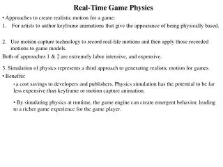
Why Physics? The Human Experience Real-world motions are physically-based Physics can make simulated game worlds appear more natural Makes sense to strive for physically-realistic motion for some types of games Emergent Behavior Physics simulation can enable a richer gaming experience
Why Physics? Developer/Publisher Cost Savings Classic approaches to creating realistic motion: Artist-created keyframe animations Motion capture Both are labor intensive and expensive Physics simulation: Motion generated by algorithm Theoretically requires only minimal artist input Potential to substantially reduce content development cost
High-level Decisions Physics in Digital Content Creation Software: Many DCC modeling tools provide physics Export physics-engine-generated animation as keyframe data Enables incorporation of physics into game engines that do not support real-time physics Straightforward update of existing asset creation pipelines Does not provide player with the same emergent-behavior-rich game experience Does not provide full cost savings to developer/publisher
High-level Decisions Real-time Physics in Game at Runtime: Enables the emergent behavior => a richer game experience Potential cost savings to developer May require significant upgrade of game engine May require significant update of asset creation pipelines May require special training for modelers, animators, and level designers Licensing an existing engine may significantly increase third party costs
High-level Decisions License vs. Build Physics Engine: License middleware physics engine Complete solution from day 1 Proven, robust code base (in theory) Most offer some integration with DCC tools Features are always a tradeoff
High-level Decisions License vs. Build Physics Engine: Build physics engine in-house Choose only the features you need Opportunity for more game-specific optimizations Greater opportunity to innovate Cost can be easily be much greater No asset pipeline at start of development
The Beginning: Particle Physics Real-time Game Physics
The Beginning: Particle Physics What is a Particle? A sphere of finite radius with a perfectly smooth, frictionless surface Experiences no rotational motion Particle Kinematics Defines the basic properties of particle motion Position, Velocity, Acceleration
Particle Kinematics - Position • Location of Particle in World Space • SI Units: meters (m) • Changes over time when object moves
Particle Kinematics - Velocity and Acceleration • Velocity (SI units: m/s) • First time derivative of position: • Acceleration (SI units: m/s2) • First time derivative of velocity • Second time derivative of position
Newton’s 2nd Law of Motion Paraphrased – “An object’s change in velocity is proportional to an applied force” The Classic Equation: m = mass (SI units: kilograms, kg) F(t) = force (SI units: Newtons)
What is Physics Simulation? The Cycle of Motion: Force, F(t), causes acceleration Acceleration, a(t), causes a change in velocity Velocity, V(t) causes a change in position Physics Simulation: Solving variations of the above equations over time to emulate the cycle of motion
Example: 3D Projectile Motion Constant Force Weight of the projectile, W = mg g is constant acceleration due to gravity Closed-form Projectile Equations of Motion: These closed-form equations are valid, and exact*, for any time, t, in seconds, greater than or equal to tinit
Example: 3D Projectile Motion Initial Value Problem Simulation begins at time tinit The initial velocity, Vinit and position, pinit, at time tinit, are known Solve for later values at any future time, t, based on these initial values On Earth: If we choose positive Z to be straight up (away from center of Earth), gEarth = 9.81 m/s2:
Concrete Example: Target Practice Projectile Launch Position, pinit Target
Concrete Example: Target Practice • Choose Vinit to Hit a Stationary Target • ptarget is the stationary target location • We would like to choose the initial velocity, Vinit, required to hit the target at some future time, thit. • Here is our equation of motion at time thit: • Solution in general is a bit tedious to derive… • Infinite number of solutions! • Hint: Specify the magnitude of Vinit, solve for its direction
Concrete Example: Target Practice • Choose Scalar launch speed, Vinit, and Let: • Where:
Concrete Example: Target Practice • If Radicand in tan Equation is Negative: • No solution. Vinitis too small to hit the target • Otherwise: • One solution if radicand == 0 • If radicand > 0, TWO possible launch angles, • Smallest yields earlier time of arrival, thit • Largest yields later time of arrival, thit
Target Practice – A Few Examples Vinit = 25 m/s Value of Radicand of tan equation: Launch angle : 19.4 deg or 70.6 deg 969.31
Target Practice – A Few Examples Vinit = 20 m/s Value of Radicand of tan equation: Launch angle : 39.4 deg or 50.6 deg 60.2
Target Practice – A Few Examples Vinit = 19.85 m/s Value of Radicand of tan equation: Launch angle : 42.4 deg or 47.6 deg (note convergence) 13.2
Target Practice – A Few Examples Vinit = 19 m/s Value of Radicand of tan equation: Launch angle : No solution! Vinit too small to reach target! -290.4
Target Practice – A Few Examples Vinit = 18 m/s Value of Radicand of tan equation: Launch angle : -6.38 deg or 60.4 deg 2063
Target Practice – A Few Examples Vinit = 30 m/s Value of Radicand of tan equation: Launch angle : 39.1 deg or 75.2 deg 668
Practical Implementation: Numerical Simulation Real-time Game Physics
What is Numerical Simulation? Equations Presented Above They are “closed-form” Valid and exact for constant applied force Do not require time-stepping Just determine current game time, t, using system timer e.g., t = QueryPerformanceCounter / QueryPerformanceFrequency or equivalent on Microsoft® Windows® platforms Plug t and tinit into the equations Equations produce identical, repeatable, stable results, for any time, t, regardless of CPU speed and frame rate
What is Numerical Simulation? The above sounds perfect Why not use those equations always? Constant forces aren’t very interesting Simple projectiles only Closed-form solutions rarely exist for interesting (non-constant) forces We need a way to deal when there is no closed-form solution… Numerical Simulation represents a series of techniques for incrementally solving the equations of motion when forces applied to an object are not constant, or when otherwise there is no closed-form solution
Finite Difference Methods What are They? The most common family of numerical techniques for rigid-body dynamics simulation Incremental “solution” to equations of motion Derived using truncated Taylor Series expansions See text for a more detailed introduction “Numerical Integrator” This is what we generically call a finite difference equation that generates a “solution” over time
Finite Difference Methods The Explicit Euler Integrator: Properties of object are stored in a state vector, S Use the above integrator equation to incrementally update S over time as game progresses Must keep track of prior value of S in order to compute the new For Explicit Euler, one choice of state and state derivative for particle:
Explicit Euler Integration Vinit = 30 m/s Launch angle, : 75.2 deg (slow arrival) Launch angle, : 0 deg (motion in world xz plane) Mass of projectile, m: 2.5 kg Target at <50, 0, 20> meters tinit pinit mVinit Vinit F=Weight = mg S = <mVinit, pinit > dS/dt = <mg,Vinit>
Explicit Euler Integration t = .2 s t = .1 s t = .01 s
A Tangent: Truncation Error The previous slide highlights values in the numerical solution that are different from the exact, closed-form solution This difference between the exact solution and the numerical solution is primarily truncation error Truncation error is equal and opposite to the value of terms that were removed from the Taylor Series expansion to produce the finite difference equation Truncation error, left unchecked, can accumulate to cause simulation to become unstable This ultimately produces floating point overflow Unstable simulations behave unpredictably
A Tangent: Truncation Error Controlling Truncation Error Under certain circumstances, truncation error can become zero, e.g., the finite difference equation produces the exact, correct result For example, when zero force is applied More often in practice, truncation error is nonzero Approaches to control truncation error: Reduce time step, t Select a different numerical integrator See text for more background information and references
Explicit Euler Integration – Truncation Error Lets Look at Truncation Error (position only) Truncation Error
Explicit Euler Integration – Truncation Error (1/t) * Truncation Error is a linear (first-order) function of t: explicit Euler Integration is First-Order-Accurate in time This accuracy is denoted by “O(t)”
Explicit Euler Integration - Computing Solution Over Time The solution proceeds step-by-step, each time integrating from the prior state
Finite Difference Methods • The Verlet Integrator: • Must store state at two prior time steps, S(t) and S(t-t) • Uses second derivative of state instead of the first • Valid for constant time step only (as shown above) • For Verlet, choice of state and state derivative for a particle:
Verlet Integration • Since Verlet requires two prior values of state, S(t) and S(t-t), you must use some method other than Verlet to produce the first numerical state after start of simulation, S(tinit+t) • Solution: Use explicit Euler integration to produce S(tinit+t), then Verlet for all subsequent time steps p a=<0,0,-g> S = <p> d2S/dt2 = <a>
Verlet Integration • The solution proceeds step-by-step, each time integrating from the prior two states • For constant acceleration, Verlet integration produces results identical to those of explicit Euler • But, results are different when non-constant forces are applied • Verlet Integration tends to be more stable than explicit Euler for generalized forces S(t-t) S(t) S(t+t)
Generalized Rigid Bodies Real-time Game Physics
Generalized Rigid Bodies • Key Differences from Particles • Not necessarily spherical in shape • Position, p, represents object’s center-of-mass location • Surface may not be perfectly smooth • Friction forces may be present • Experience rotational motion in addition to translational (position only) motion
Generalized Rigid Bodies – Simulation • Angular Kinematics • Orientation, 3x3 matrix R or quaternion, q • Angular velocity, • As with translational/particle kinematics, all properties are measured in world coordinates • Additional Object Properties • Inertia tensor, J • Center-of-mass • Additional State Properties for Simulation • Orientation • Angular momentum, L=J • Corresponding state derivatives
Generalized Rigid Bodies - Simulation • Torque • Analogous to a force • Causes rotational acceleration • Cause a change in angular momentum • Torque is the result of a force (friction, collision response, spring, damper, etc.)
Generalized Rigid Bodies – Numerical Simulation • Using Finite Difference Integrators • Translational components of state <mV, p> are the same • S and dS/dt are expanded to include angular momentum and orientation, and their derivatives • Be careful about coordinate system representation for J, R, etc. • Otherwise, integration step is identical to the translation only case • Additional Post-integration Steps • Adjust orientation for consistency • Adjust updated R to ensure it is orthogonal • Normalize q • Update angular velocity, • See text for more details
Collision Response • Why? • Performed to keep objects from interpenetrating • To ensure behavior similar to real-world objects • Two Basic Approaches • Approach 1: Instantaneous change of velocity at time of collision • Benefits: • Visually the objects never interpenetrate • Result is generated via closed-form equations, and is perfectly stable • Difficulties: • Precise detection of time and location of collision can be prohibitively expensive (frame rate killer) • Logic to manage state is complex
Collision Response • Two Basic Approaches (continued) • Approach 2: Gradual change of velocity and position over time, following collision • Benefits • Does not require precise detection of time and location of collision • State management is easy • Potential to be more realistic, if meshes are adjusted to deform according to predicted interpenetration • Difficulties • Object interpenetration is likely, and parameters must be tweaked to manage this • Simulation can be subject to numerical instabilities, often requiring the use of implicit finite difference methods
Final Comments • Instantaneous Collision Response • Classical approach: Impulse-momentum equations • See text for full details • Gradual Collision Response • Classical approach: Penalty force methods • Resolve interpenetration over the course of a few integration steps • Penalty forces can wreak havoc on numerical integration • Instabilities galore • Implicit finite difference equations can handle it • But more difficult to code • Geometric approach: Ignore physical response equations • Enforce purely geometric constraints once interpenetration has occurred