Antenna Patterns and Antenna Parameters
Antenna Patterns and Antenna Parameters. Prepared by Muhammad Mostafa Amir Faisal. Antenna. Antenna Field Regions. The fields surrounding an antenna are divided into 3 principle regions: Reactive Near Field Radiating Near Field or Fresnel Region

Antenna Patterns and Antenna Parameters
E N D
Presentation Transcript
Antenna Patterns and Antenna Parameters Prepared by Muhammad Mostafa Amir Faisal
Antenna Field Regions The fields surrounding an antenna are divided into 3 principle regions: • Reactive Near Field • Radiating Near Field or Fresnel Region • Far Field or Fraunhofer Region The far field region is the most important, as this determines the antenna's radiation pattern. Also, antennas are used to communicate wirelessly from long distances, so this is the region of operation for most antennas.
Far Field (Fraunhofer) Region • The far field is the region far from the antenna, as you might suspect. In this region, the radiation pattern does not change shape with distance (although the fields still die off as 1/R, the power density dies off as 1/R^2). Also, this region is dominated by radiated fields, with the E- and H-fields orthogonal to each other and the direction of propagation as with plane waves. • If the maximum linear dimension of an antenna is D, then the following 3 conditions must all be satisfied to be in the far field region: • Eqns:
Reactive Near Field Region • In the immediate vicinity of the antenna, we have the reactive near field. In this region, the fields are predominately reactive fields, which means the E- and H- fields are out of phase by 90 degrees to each other (recall that for propagating or radiating fields, the fields are orthogonal (perpendicular) but are in phase). • The boundary of this region is commonly given as: • d
Radiating Near Field (Fresnel) Region • The radiating near field or Fresnel region is the region between the near and far fields. In this region, the reactive fields are not dominate; the radiating fields begin to emerge. However, unlike the Far Field region, here the shape of the radiation pattern may vary appreciably with distance.The region is commonly given by: • d
Antenna or Radiation Pattern • An antenna radiation pattern or antenna pattern is defined as “a mathematical function or a graphical representation of the radiation properties of the antenna as a function of space coordinates. • In most cases, the radiation pattern is determined in the far field region and is represented as a function of the directional coordinates. Radiation properties include power flux density, radiation intensity, field strength, directivity, phase or polarization.” • The radiation property of most concern is the two- or three dimensional spatial distribution of radiated energy as a function of the observer’s position along a path or surface of constant radius.
Some definations • The main beam is the region around the direction of maximum radiation (usually the region that is within 3 dB of the peak of the main beam). The main beam in Figure 2 is centered at 90 degrees. • The sidelobes are smaller beams that are away from the main beam. These sidelobes are usually radiation in undesired directions which can never be completely eliminated. The sidelobes in Figure 2 occur at roughly 45 and 135 degrees. • The Half Power Beamwidth (HPBW) is the angular separation in which the magnitude of the radiation pattern decrease by 50% (or -3 dB) from the peak of the main beam. From Figure 2, the pattern decreases to -3 dB at 77.7 and 102.3 degrees. Hence the HPBW is 102.3-77.7 = 24.6 degrees. • Another commonly quoted beamwidth is the Null to Null Beamwidth. This is the angular separation from which the magnitude of the radiation pattern decreases to zero (negative infinity dB) away from the main beam. From Figure 2, the pattern goes to zero (or minus infinity) at 60 degrees and 120 degrees. Hence, the Null-Null Beamwidth is 120-60=60 degrees.
Reflection Co-efficient or S-11 parameter • In practice, the most commonly quoted parameter in regards to antennas is S11. S11 represents how much power is reflected from the antenna, and hence is known as the reflection coefficient (sometimes written as gamma: or return loss. If S11=0 dB, then all the power is reflected from the antenna and nothing is radiated. If S11=-10 dB, this implies that if 3 dB of power is delivered to the antenna, -7 dB is the reflected power. The remainder of the power was "accepted by" or deliverd to the antenna. This accepted power is either radiated or absorbed as losses within the antenna. Since antennas are typically designed to be low loss,
S11 from graph • The above figure implies that the antenna radiates best at 2.5 GHz, where S11=-10 dB. Further, at 1.5 GHz the antenna will radiate virtually nothing, as S11 is close to 0 dB (so all the power is reflected). The antenna bandwidth can also be determined from the above figure. If the bandwidth is defined as the frequency range where S11 is to be less than -6 dB, then the bandwidth would be roughly 1 GHz, with 3 GHz the high end and 2 GHz the low end of the frequency band.
VSWR • The VSWR is always a real and positive number for antennas. The smaller the VSWR is, the better the antenna is matched to the transmission line and the more power is delivered to the antenna. The minimum VSWR is 1.0. In this case, no power is reflected from the antenna, which is ideal. • Often antennas must satisfy a bandwidth requirement that is given in terms of VSWR. For instance, an antenna might claim to operate from 100-200 MHz with VSWR<3. This implies that the VSWR is less than 3.0 over the specified frequency range. This VSWR specifications also imples that the reflection coefficient is less than 0.5 (i.e., <0.5) over the quoted frequency range.
UNDERSTANDING VSWR • Is a VSWR of 3 bad? How bad is a VSWR of 12? • In the above table, a VSWR of 4 has 36% of power delivered by the receiver reflected from the antenna (64% of the power is delivered to the antenna). Note that a reflected power of 0 dB indicates all of the power is reflected (100%), whereas -10 dB indicates 10% of the power is reflected. If all the power is reflected, the VSWR would be infinite. • In general, if the VSWR is under 2 the antenna match is considered very good and little would be gained by impedance matching. As the VSWR increases, there are 2 main negatives. The first is obvious: more power is reflected from the antenna and therefore not transmitted. However, another problem arises. As VSWR increases, more power is reflected to the radio, which is transmitting. Large amounts of reflected power can damage the radio. In addition, radios have trouble transmitting the correct information bits when the antenna is poorly matched (this is numerically defined in terms of another metric, EVM - Error Vector Magnitude).
Fractional Bandwidth • The fractional bandwidth of an antenna is a measure of how wideband the antenna is. If the antenna operates at center frequency fc between lower frequency f1 and upper frequency f2 (where fc=(f1+f2)/2), then the fractional bandwidth FBW is given by: • The fractional bandwidth varies between 0 and 2, and is often quoted as a percentage (between 0% and 200%). The higher the percentage, the wider the bandwidth. • Wideband antennas typically have a Fractional Bandwidth of 20% or more. Antennas with a FBW of greater than 50% are referred to as ultra-wideband antennas.
POLARIZATION • The polarization of waves refer to the time varying behavior of the electric field strength vector at some fixed point. The polarization of waves is the locus of the tip of the electric field of a given point as a function of time. • Polarization of antenna refers to the polarization of the electric field vector of the radiated wave.
Types of Polarization • Linear Polarization: A wave is said to be linearly polarized when some point in the medium, electric field oscillates along a straight line. • Circular Polarization: A wave is said to be ciecularly polarized at some point in space if the electric field traces a circular path as a function of time • Elliptical Polarization: Ellipse(just elliptical in place of circular)
How to understand! • A plane electromagnetic (EM) wave is characterized by travelling in a single direction (with no field variation in the two orthogonal directions). In this case, the electric field and the magnetic field are perpendicular to each other and to the direction the plane wave is propagating. • As an example, consider the single frequency E-field given by equation (1), where the field is traveling in the +z-direction, the E-field is oriented in the +x-direction, and the magnetic field is in the +y-direction.
Linear • Polarization is the figure that the E-field traces out while propagating. As an example, consider the E-field observed at (x,y,z)=(0,0,0) as a function of time for the plane wave described by equation (1) above. The amplitude of this field is plotted in Figure 2 at several instances of time. The field is oscillating at frequency f.
Contnd.. • Observed at the origin, the E-field oscillates back and forth in magnitude, always directed along the x-axis. Because the E-field stays along a single line, this field would be said to be linearly polarized. In addition, if the x-axis was parallel to the ground, this field could also be described as "horizontally polarized" (or sometimes h-pole in the industry). If the field was oriented along the y-axis, this wave would be said to be "vertically polarized" (or v-pole).
Contnd.. • A linearly polarized wave does not need to be along the horizontal or vertical axis. For instance, a wave with an E-field constrained to lie along the line shown in Figure 3 would also be linearly polarized. • The E-field in Figure 3 could be described by equation (2). The E-field now has an x- and y- component, equal in magnitude.
Conditions • Only one component • Two linear orthogonal components that are in time phase or 180 degree out of phase
Circular Polarization • Suppose now that the E-field of a plane wave was given by equation (3): • In this case, the x- and y- components are 90 degrees out of phase. If the field is observed at (x,y,z)=(0,0,0) again as before, the plot of the E-field versus time would appear as shown in Figure 4.
Criteria for Circular Polarization • The E-field must have two orthogonal (perpendicular) components. • The E-field's orthogonal components must have equal magnitude. • The orthogonal components must be 90 degrees out of phase.
Additional • If the wave in Figure 4 is travelling out of the screen, the field is rotating in the counter-clockwise direction and is said to be Right Hand Circularly Polarized (RHCP). If the fields were rotating in the clockwise direction, the field would be Left Hand Circularly Polarized (LHCP).
Elliptical Polarization • If the E-field has two perpendicular components that are out of phase by 90 degrees but are not equal in magnitude, the field will end up Elliptically Polarized. Consider the plane wave travelling in the +z-direction, with E-field described by equation (4):
conclusion • The field in Figure 5, travels in the counter-clockwise direction, and if travelling out of the screen would be Right Hand Elliptically Polarized. If the E-field vector was rotating in the opposite direction, the field would be Left Hand Elliptically Polarized.In addition, elliptical polarization is defined by its eccentricity, which is the ratio of the major and minor axis amplitudes. For instance, the eccentricity of the wave given by equation (4) is 1/0.3 = 3.33. Elliptically polarized waves are further described by the direction of the major axis. The wave of equation (4) has a major axis given by the x-axis. Note that the major axis can be at any angle in the plane, it does not need to coincide with the x-, y-, or z-axis. Finally, note that circular polarization and linear polarization are both special cases of elliptical polarization. An elliptically polarized wave with an eccentricity of 1.0 is a circularly polarized wave; an elliptically polarized wave with an infinite eccentricity is a linearly polarized wave.
Criteria? • homework
Receiving AntennaReciprocity Theorem • Reciprocity is one of the most useful (and fortunate) property of antennas. Reciprocity states that the receive and transmit properties of an antenna are identical. Hence, antennas do not have distinct transmit and receive radiation patterns - if you know the radiation pattern in the transmit mode then you also know the pattern in the receive mode. This makes things much simpler, as you can imagine. (note)
Polarization of Antennas • The polarization of an antenna is the polarization of the radiated fields produced by an antenna, evaluated in the far field. Hence, antennas are often classified as "Linearly Polarized" or a "Right Hand Circularly Polarized Antenna". • This simple concept is important for antenna to antenna communication. First, a horizontally polarized antenna will not communicate with a vertically polarized antenna. Due to the reciprocity theorem, antennas transmit and receive in exactly the same manner. Hence, a vertically polarized antenna transmits and receives vertically polarized fields. Consequently, if a horizontally polarized antenna is trying to communicate with a vertically polarized antenna, there will be no reception.
PLF • In general, for two linearly polarized antennas that are rotated from each other by an angle , the power loss due to this polarization mismatch will be described by the Polarization Loss Factor (PLF): • Hence, if both antennas have the same polarization, the angle between their radiated E-fields is zero and there is no power loss due to polarization mismatch. If one antenna is vertically polarized and the other is horizontally polarized, the angle is 90 degrees and no power will be transferred. • As a side note, this explains why moving the cell phone on your head to a different angle can sometimes increase reception. Cell phone antennas are often linearly polarized, so rotating the phone can often match the polarization of the phone and thus increase reception.
Circular polarization is a desirable characteristic for many antennas. Two antennas that are both circularly polarized do not suffer signal loss due to polarization mismatch. Antennas used in GPS systems are Right Hand Circularly Polarized. • Suppose now that a linearly polarized antenna is trying to receive a circularly polarized wave. Equivalently, suppose a circularly polarized antenna is trying to receive a linearly polarized wave. What is the resulting Polarization Loss Factor? • Recall that circular polarization is really two orthongal linear polarized waves 90 degrees out of phase. Hence, a linearly polarized (LP) antenna will simply pick up the in-phase component of the circularly polarized (CP) wave • The Polarization Loss Factor is sometimes referred to as polarization efficiency, antenna mismatch factor, or antenna receiving factor. All of these names refer to the same concept.
Aperture Area • A useful parameter calculating the receive power of an antenna is the effective area or effective aperture. Assume that a plane wave with the same polarization as the receive antenna is incident upon the antenna. Further assume that the wave is travelling towards the antenna in the antenna's direction of maximum radiation (the direction from which the most power would be received). • Then the effective aperture parameter describes how much power is captured from a given plane wave. Let p be the power density of the plane wave (in W/m^2). If P_t represents the power (in Watts) at the antennas terminals available to the antenna's receiver,
Hence, the effective area simply represents how much power is captured from the plane wave and delivered by the antenna. This area factors in the losses intrinsic to the antenna (ohmic losses, dielectric losses, etc.). • A general relation for the effective aperture in terms of the peak antenna gain (G) of any antenna is given by:
Effective Length • It shows the effectiveness of an antenna as a radiator or collector of EM wave energy. • Effective length= Open Ckt Voltage/ Incident Electric Field Strength
Friis Free Space Equation • The Friis Transmission Equation is used to calculate the power received from one antenna (with gain G1), when transmitted from another antenna (with gain G2), separated by a distance R, and operating at frequency f or wavelength lambda. The Friis Transmission Equation is used to calculate the power received from one antenna (with gain G1), when transmitted from another antenna (with gain G2), separated by a distance R, and operating at frequency f or wavelength lambda. • To begin the derivation of the Friis Equation, consider two antennas in free space (no obstructions nearby) separated by a distance R: Figure 1. Transmit (Tx) and Receive (Rx) Antennas separated by R.
Contnd… • Assume that Watts of total power are delivered to the transmit antenna. For the moment, assume that the transmit antenna is omnidirectional, lossless, and that the receive antenna is in the far field of the transmit antenna. Then the power density p (in Watts per square meter) of the plane wave incident on the receive antenna a distance R from the transmit antenna is given by:
If the transmit antenna has an antenna gain in the direction of the receive antenna given by , then the power density equation above becomes: • The gain term factors in the directionality and losses of a real antenna. Assume now that the receive antenna has an effective aperture given by . Then the power received by this antenna ( ) is given by:
Since the effective aperture for any antenna can also be expressed as: • The resulting received power can be written as: • This is known as the Friis Transmission Formula. It relates the free space path loss, antenna gains and wavelength to the received and transmit powers. This is one of the fundamental equations in antenna theory, and should be remembered (as well as the derivation above).
Another useful form of the Friis Transmission Equation is given in Equation [2]. Since wavelength and frequency f are related by the speed of light c,we have the Friis Transmission Formula in terms of frequency: ( 2) • Equation [2] shows that more power is lost at higher frequencies. This is a fundamental result of the Friis Transmission Equation. This means that for antennas with specified gains, the energy transfer will be highest at lower frequencies. The difference between the power received and the power transmitted is known as path loss. Said in a different way, Friis Transmission Equation says that the path loss is higher for higher frequencies.
This is why mobile phones generally operate at less than 2 GHz. • The importance of this result from the Friis Transmission Formula cannot be overstated. This is why mobile phones generally operate at less than 2 GHz. There may be more frequency spectrum available at higher frequencies, but the associated path loss will not enable quality reception. • As a further consequence of Friss Transmission Equation, suppose you are asked about 60 GHz antennas. Noting that this frequency is very high, you might state that the path loss will be too high for long range communication - and you are absolutely correct. At very high frequencies (60 GHz is sometimes referred to as the mm (millimeter wave) region), the path loss is very high, so only point-to-point communication is possible. This occurs when the receiver and transmitter are in the same room, and facing each other. • As a further corrollary of Friis Transmission Formula, do you think the mobile phone operators are happy about the new LTE (4G) band, that operates at 700MHz? The answer is yes: this is a lower frequency than antennas traditionally operate at, but from Equation [2], we note that the path loss will therefore be lower as well. Hence, they can "cover more ground" with this frequency spectrum, • Side Note: On the other hand, the cell phone makers will have to fit an antenna with a larger wavelength in a compact device (lower frequency = larger wavelength), so the antenna designer's job got a little more complicated!
Finally, if the antennas are not polarization matched, the above received power could be multiplied by the Polarization Loss Factor (PLF) to properly account for this mismatch. Equation [2] above can be altered to produce a generalized Friis Transmission Formula, which includes polarization mismatch:
Decibel Math • To convert Friis Transmission equation from linear units in Watts to decibels, we take the logarithm of both sides and multiply by 10 • A nice property of logarithms is that for two numbers A and B (both positive), the following result is always true: • Equation Becomes:
Using the definition of decibels, the above equation becomes a simple addition equation in dB: • The above representation is easier to work with.