Download
1 / 35
350 likes | 563 Views
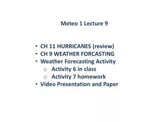
Meteo 1 Lecture 9 CH 11 HURRICANES (review) CH 9 WEATHER FORCASTING Weather Forecasting Activity Activity 6 in class Activity 7 homework Video Presentation and Paper. REVIEW SLIDES:.

E N D
Meteo 1 Lecture 9 • CH 11 HURRICANES (review) • CH 9 WEATHER FORCASTING • Weather Forecasting Activity • Activity 6 in class • Activity 7 homework • Video Presentation and Paper
REVIEW SLIDES: Hurricane Elena over the Gulf of Mexico about 130 km (80 mi) southwest of Apalachicola, Florida, as photographed from the space shuttle Discovery during September, 1985. Because this storm is situated north of the equator, surface winds are blowing counterclockwise about its center (eye). The central pressure of the storm is 955 mb, with sustained winds of 105 knots (121 mi/hr) near its eye.
REVIEW SLIDES: intensifying tropical cyclone air pressure drops rapidly as you approach the eye of the storm surface winds normally reach maximum strength in the region of the eyewall
REVIEW SLIDES: Visible satellite image showing four tropical systems, each in a different stage of development.
REVIEW SLIDES: Regions where tropical storms form (orange shading), the names given to storms, and the typical paths they take (red arrows).
Meteo 1 Lecture 9 • CH 9 WEATHER FORCASTING • Acquisition of Weather Data • Weather Forecasting Methods • Types of Forecasts • Weather Forecasting Using Surface Charts First, lets review some of the meteorologic factors that contribute to weather: http://ww2010.atmos.uiuc.edu/%28Gh%29/guides/mtr/fcst/home.rxml
A sounding of air temperature, dew point, and winds at Pittsburgh, PA, on January 14, 1999.
The geostationary satellite moves through space at the same rate that the earth rotates, so it remains above a fixed spot on the equator and monitors one area constantly.
Polar-orbiting satellites scan from north to south, and on each successive orbit the satellite scans an area farther to the west.
Generally, the lower the cloud, the warmer its top. Warm objects emit more infrared energy than do cold objects. Thus, an infrared satellite picture can distinguish warm, low (gray) clouds from cold, high (white) clouds.
Weather Forecasting Methods First, lets preview some of the forecasting methods: • Why Forecasts Go Awry • Assumptions • Models not global • Regions with few observations • Cannot model small-scale features • All factors cannot be modeled • Ensemble Forecasts: • Spaghetti model, robust • Observation: Weathercasters • Chroma key or color separation http://ww2010.atmos.uiuc.edu/%28Gh%29/guides/mtr/fcst/mth/prst.rxml
Two 500-mb progs for 7 p.m. EST, July 12, 2006 — 48 hours into the future. Prog (a) is the WRF/NAM model, with a resolution (grid spacing) of 12 km, whereas prog (b) is the GFS model with a resolution of 60 km. Solid lines on each map are height contours, where 570 equals 5700 meters. Notice how the two progs (models) agree on the atmosphere’s large scale circulation. The main difference between the progs is in the way the models handle the low off the west coast of North America.
Model (a) predicts that the low will dig deeper along the coast
model (b) predicts a more elongated west-to-east (zonal) low.
Ensemble 500-mb forecast chart for July 21, 2005 (48 hours into the future). The chart is constructed by running the model 15 different times, each time beginning with a slightly different initial condition. The blue lines represent the 5790-meter contour line; the red lines, the 5940-meter contour line; and the green line, the 500-mb 25-year average, called climatology.
Probability of a “White Christmas”—one inch or more of snow on the ground—based on a 30-year average. The probabilities do not include all of the mountainous areas in the western United States. (NOAA)
The 90-day outlook for (a) precipitation and (b) temperature for February, March, and April, 2011.
For precipitation (a), the darker the green color the greater the probability of precipitation being above normal, whereas the deeper the brown color the greater the probability of precipitation being below normal.
For temperature (b), the darker the orange/red colors the greater the probability of temperatures being above normal, whereas the darker the blue color, the greater the probability of temperatures being below normal.
Weather Forecasting Using Surface Charts Movement of Weather Systems, some generalizations: • Mid-lat cyclones move in same direction and speed as previous 6 hrs • Lows move in direction parallel the isobars in the warm air ahead of the cold front • Lows move toward region of greatest pressure drop
Surface weather map for 6:00 a.m. Tuesday. Dashed lines indicate positions of weather features six hours ago. Areas shaded green are receiving rain, while areas shaded white are receiving snow, and those shaded pink, freezing rain or sleet. BONUS SLIDE
A 500-mb chart for 6:00 a.m. Tuesday, showing wind flow. The light orange L represents the position of the surface low. The winds aloft tend to steer surface pressure systems along and, therefore, indicate that the surface low should move northeastward at about half the speed of the winds at this level, or 25 knots. Solid lines are contours in meters above sea level. BONUS SLIDE
Projected 12- and 24-hour movement of fronts, pressure systems, and precipitation from 6:00 a.m. Tuesday until 6:00 a.m. Wednesday. (The dashed lines represent frontal positions 6 hours ago.) BONUS SLIDE
Surface weather map for 6:00 a.m. Wednesday. BONUS SLIDE
Forecast on your own! BONUS SLIDE
Meteo 1 Lecture 9 • CH 9 WEATHER FORCASTING • Acquisition of Weather Data • Weather Forecasting Methods • Types of Forecasts • Weather Forecasting Using Surface Charts
Weather Map Activity 6 • 30 Points • Launch other Presentation
Weather Forecast Activity 7 • 30 Points • Homework to forecast the weather and test one’s forecast
Meteo 1 Fall 2012 Activity 7 Weather Forecasting (2 parts) 30 points! Part 1 Forecast: Prepare a weather forecast for two cities (one on the west coast and one on the interior, like Utah, Colorado, or Kansas). The forecast may be completed at any time before our next class. The forecast and the Part 2 comparison need to be submitted the day before the intended forecast day (eg. if one is forecasting the weather on Wednesday, then one needs to submit the forecast before midnight of the night between Tuesday and Wednesday). The forecast consists of the following elements: *During the period from midnight - 11:59 PM, local time City 1 Coastal ________________________ Maximum temperature* Justification for your maximum temperature forecast Minimum temperature* Justification for your minimum temperature forecast Wind speed at noon Justification for your wind speed forecast Wind direction at noon Justification for your wind direction forecast Homework Activity Source: https://pantherfile.uwm.edu/kahl/www/Forecast/
NWS: monthly and seasonal outlook maps: http://www.cpc.ncep.noaa.gov/products/predictions/multi_season/13_seasonal_outlooks/color/churchill.php NWS Hydrometeorological Prediction Center http://www.hpc.ncep.noaa.gov/ Learning lesson: drawing conclusions: http://www.srh.noaa.gov/jetstream/synoptic/ll_analyze.htm jetstream online school for weather: http://www.srh.noaa.gov/jetstream/synoptic/synoptic_intro.htm NOAA Environmental Visualization Gallery: http://www.nnvl.noaa.gov/Atmosphere.php