Graphical Solutions
This guide explores graphical solutions to linear programming problems, encompassing the plotting of constraints, identification of the feasible region, and optimization methods. It explains the nature of feasible regions, including scenarios of infeasibility and unbounded solutions. The two methods for finding optimal solutions—level curves and extreme points—are detailed, illustrating how to use graphical techniques for optimization. Additionally, it highlights common solver messages and potential issues encountered while solving linear programming problems.

Graphical Solutions
E N D
Presentation Transcript
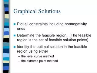
Graphical Solutions • Plot all constraints including nonnegativity ones • Determine the feasible region. (The feasible region is the set of feasible solution points) • Identify the optimal solution in the feasible region using either • the level curve method • the extreme point method
Feasible Regions • The feasible region for a two-variable linear programming problem can be nonexistent, a single point, a line, a polygon, or an unbounded area. • If a constraint can be removed without affecting the shape of the feasible region, the constraint is said to be redundant. • An overconstrained LP that does not have one point satisfying all the constraints simultaneously is said to be infeasible and a feasible region does not exist. • The feasible region for the KPiller problem is a polygon, illustrating that an infinite number of feasible solutions exist for this problem. (See class handout). • Assuming that a feasible region exists, an optimal solution will always occur at one or more of the extreme points, where an extreme point is a corner point of the feasible region.
Level Curves • Plot a level curve for a targeted objective function value • Level curves are parallel lines that shift away from the origin as the targeted objective function value increases • Slide the level curve in the direction of improvement (away from the origin if maximizing, toward the origin if minimizing) until it reaches the last point where it still touches at least one point in the feasible region • Solve the two equations which specify the identified feasible point to determine the optimal solution
Determine all of the extreme points of the feasible region: Extreme Point (3.5, 3) (6.5, 3) (4.5, 7) (1.5, 9) Calculate the resulting objective function value for each point: Z = 5000*E9 + 4000*F9 $29,500 $44,500 $50,500 $43,500 Extreme Point Method
Types of LP Solutions • Any linear program falls in one of three categories: • is infeasible • has a unique optimal solution or alternate optimal solutions • has an objective function that can be increased without bound • In the graphical method, if the objective function line is parallel to a boundary constraint in the direction of optimization, there are alternate optimal solutions, with all points on this line segment being optimal.
Solver Result Messages • Solver found a solution. All constraints and optimality conditions are satisfied: Solver has correctly identified an optimal solution for the problem you have formulated. Note that there may be alternative optimal solutions possible however. • Solver has converged to the current solution. All constraints are satisfied: You have not selected the linear programming option in the Solver options. Thus nonlinear programming is being performed and this is the best solution Solver has found so far. It is not guaranteed to be the optimal one however.
Example: Infeasible Problem • Solve graphically for the optimal solution: Max z = 2x1 + 6x2 s.t. 4x1 + 3x2< 12 2x1 + x2> 8 x1, x2> 0
x2 2x1 + x2> 8 8 4x1 + 3x2< 12 4 x1 3 4 Example: Infeasible Problem • There are no points that satisfy both constraints, hence this problem has no feasible region, and no optimal solution.
Solver Result Message • Solver could not find a feasible solution Possible problems if you know the solution should be feasible are: • too many constraints in Solver • one of the constraints may be entered wrong (e.g. the inequality sign might be going the wrong way) • you may not have the correct changing cells (decision variables) specified in Solver • one or more formulas in the spreadsheet may have been erased.
Example: Unbounded Problem • Solve graphically for the optimal solution: Max z = 3x1 + 4x2 s.t. x1 + x2> 5 3x1 + x2> 8 x1, x2> 0
x2 3x1 + x2> 8 8 x1 + x2> 5 5 Max 3x1 + 4x2 x1 2.67 5 Example: Unbounded Problem • The feasible region is unbounded and the objective function line can be moved parallel to itself without bound so that z can be increased infinitely.
Solver Result Messages • Set Cell values do not converge: Your model as formulated is unbounded. • One or more constraint is missing from the problem or entered wrong (e.g. an inequality sign is in the wrong direction). • Often times the modeler has forgotten to check the Assume Nonnegativity option in Solver. Note: A feasible region may be unbounded and yet there may be optimal solutions. In the case where the objective does not move in the direction of the unboundedness, you will see the optimal Solver solution message instead of this message.
Solver Result Messages • The linearity conditions required by this LP Solver are not satisfied: Solver’s preliminary tests indicate that your model is not linear. • Check for use of functions such as IF, MAX, PV, VLOOKUP which create linearity problems. Write the algebraic logic programmed in the objective and constraint cells on paper to ensure linear relationships. • Sometimes this message occurs due to poor scaling (see text section 3.11). If you think your model is linear, try resolving the model again. Often times Solver can find the solution the second time. If not, use the Use Automatic Scaling option in Solver. Solver will attempt to rescale your data. If that doesn’t work, rescale the data yourself.