Example Project Location
Sacramento Metropolitan AQMD Roadways Modeling using CAL3QHCR (A Line Source Model) Step-By-Step Procedure. Example Project Location. Example Project Information. By 2009, residential receptors will be located south of I-80 (at B St) in Sacramento. Caltrans peak traffic hourly count:

Example Project Location
E N D
Presentation Transcript
Sacramento Metropolitan AQMDRoadways Modelingusing CAL3QHCR (A Line Source Model)Step-By-Step Procedure
Example Project Information • By 2009, residential receptors will be located south of I-80 (at B St) in Sacramento. • Caltrans peak traffic hourly count: 11,900 vehicles hour.
Option 1- CAL3QHCR Roadway Modeling Procedure The CAL3QHCR modeling procedure requires both VMT, and grams per mile of PM10 for each hour of the day. This data is not usually available for any given road segment, but can be derived using EMFAC model results set for the “annual average mode”.
Option 1- Uncertainty Issues • This procedure may overestimate risks in that it assumes the toxicity of gasoline PM emissions = diesel PM. (Studies show this is more likely true than not.) • Additionally, it may underestimate or overestimate risks in that it assumes the Car/Truck ratio on roadways throughout the county are the same as the county average. This uncertainty can be overcome using more accurate segment specific VMT data.
Data preparation for CAL3QHCR • From CALTRANS, get road segment data representing the Peak Number of Vehicles/Hour • Run EMFAC set for Annual Average data, for each of 24 hours in a day to get: Annual Average Vehicle-Miles Traveled (VMT) Annual Average Tons PM10 emissions • Using EMFAC data, normalize the countywide VMT data, then multiply it with the Peak vehicles/hour data, to get VMT for the road segment. • Convert the EMFAC emissions to grams/hr, then divide the emissions by the hourly VMT straight from EMFAC to get a grams/VMT. Input this to CAL3QHCR.
Derivation - Annual Average Grams/VMTfor each hour of the day.
Obtain Traffic Data from Caltrans www.dot.ca.gov/hq/traffops/saferesr/traffdata/ Click on the most recent year
Find Route # Scroll down here to find the route number. This may require a phone call to CALTRANS to be certain of the Route number. (I5≠5)
Find Peak Hour Traffic Select ahead peak hour for projects north or east of the nearest milepost location. This project is just east of the E street marker.
EMFAC Inputs and Outputs EMFAC inputs: • Year: 2009 • Season: annual • Burden: standard • Output frequency: hourly (tons/hr) EMFAC outputs: • Annual Average VMT for each hour of the day (all vehicles) • PM10 exhaust emissions for each hour for ALL vehicles.
CAL3HQCR Modeling Procedure Overview • Open an example/old control file (.ctl) file, and edit it with the new file names you will be using. • Save the file with a new file name. • Edit over the example/old batch file (.bat) by right clicking and editing. • Save the file with the new name. • Edit the Input file (.inp). • Run the CAL3QHCR by double clicking on the batch file (.bat). • Identify the Highest Average Annual Concentrations in the output file (.out) for each receptor. • Calculate cancer risk levels at these locations.
Prepare the CAL3QHCR Files These files are needed to run CAL3QHCR: .ctl control file - CAL3QHCR looks to this file to find the files names that are read into the program, and outputted by the program. .bat batch file - DOS file batch command. .inp input file - contains scenario parameters. .exe executable file - performs the functions. .asc meteorology file - prepared previously.
Rename files Step 1 - Edit the control (.ctl) file • Open an example/old .ctl file and edit it with the new file names you will be using. • Save the file with a new file name. old new
edit file Step 2 - Edit the batch (.bat) file • Edit over the example/old .bat file by right clicking and editing. • Save the file with the new name. new old
Example Project’s Input File REC W1 defines the roadway edge. REC W1 will be thrown out because it is in the mixing zone.
Step 4 – Run the Model Double click the .bat file
CAL3QHCR creates the following files The .ET1 file is a copy of emissions, traffic volume, and signalization data as read from the .inp file. The .ET2 file is a preprocessed .ET1 data file. The .ILK file is the link data file.
Check for Errors…. • Open the .txt file and scroll down • “Program Terminated Normally” = we are good to go
Open the .OUT File Identify the Highest Average Annual Concentrations
Cancer Risk Calculation(Inhalation only pathway is acceptable for Diesel PM)