Download

1 / 38
450 likes | 1.03k Views
Analysis of Cross Section and Panel Data. Yan Zhang School of Economics, Fudan University CCER, Fudan University. Introductory Econometrics A Modern Approach. Yan Zhang School of Economics, Fudan University CCER, Fudan University. Analysis of Cross Section and Panel Data.

E N D
Analysis of Cross Section and Panel Data Yan Zhang School of Economics, Fudan University CCER, Fudan University
Introductory EconometricsA Modern Approach Yan Zhang School of Economics, Fudan University CCER, Fudan University
Analysis of Cross Section and Panel Data Part 3. Some Advanced Topics
Chap 13. Pooling Cross Sections across Time • Data Structure • Pooled Cross Section; Panel Data • Independently Pooled Cross Section • they consist of independently sampled observations. • 与单一随机样本的差别:在不同时点对总体抽样可能导致观测点不是同分布的(not identically distributed.) • Different intercept and slopes • Policy analysis • Panel Data • The same units • we cannot assume that the observations of longitudinal data are independently distributed across time. • Special models and methods • Differencing (remove time-constant, unobserved attributes of the units.)
Pooled Cross Sections • Pooling cross sections from different years; • Effectively analyzing the effects of a new govt. policy; • Similar to a standard cross section, except that we often need to account for secular differences in the variables across the time.
Panel or Longitudinal Data • The same cross sectional members; • To control certain unobserved Characteristic of cross sections; • To study the importance of lags in behavior or the result of decision making
13.1 Pooling Independent Cross Sections across Time • Increase the sample size • Dummy Variables • the population may have different distributions in different time periods • different intercept and slopes • Year dummy: including dummy variables for all but one year, where the earliest year in the sample is usually chosen as the base year. • The pattern of coef. on the year dummies • The change of the coef. of the key variable over time • policy analysis
Example 13.1 Has the pattern of women’s fertility Changed? • Factors on Women’s Fertility over Time? • age; education; religion; region • dependent variable: fertility rates; different period • Data: FERTIL1.RAW, which is similar to that used by Sander (1994), comes from the National Opinion Research Center’s General Social Survey for the even years from 1972 to 1984 • Interpretations • base year: 1972 • education: .128(4)=.512. • turning point of age • heteroskedasticity of error term over time? B-P test; WLS • educ? interaction effects (P. 13.7, IV) Has the effect of education on fertility rates changed over time?
The Chow Test for Structural Change Across Time • One form of the test obtains the sum of squared residuals from the pooled estimation as the restricted SSR. The unrestricted SSR is the sum of the SSRs for the two separately estimated time periods. • Another way: interacting each variable with a year dummy for one of the two years and testing for joint significance of the year dummy and all of the interaction terms. • Usually, after an allowance for intercept difference, certain slope coefficients are tested for constancy by interacting the variable of interest with year dummies.
E.g. 13.2 Changes in the return to education and the gender wage gap • Econometric Model: • nominal vs. real value • Provided the dollar amounts appear in logarithmic form and dummy variables are used for all time periods (except, of course, the base period), the use of aggregate price deflators will only affect the intercepts; none of the slope estimates will change. • Chow Test: • What happens if we interact all independent variables with y85 in equation (13.2)?
13.2 Policy Analysis with Pooled Cross Sections • natural experiments: occurs when some exogenous event—often a change in government policy—changes the environment in which individuals, families, firms, or cities operate. • control group: not affected by the policychange • treatment group: thought to be affected by the policy change. • Methods: • to control for systematic differences between the control and treatment groups, we need two years of data, one before the policy change and one after the change. • the difference-in-differences estimator:
Example 13.4 Effects of Worker Compensation Laws on Duration • 1980.7.15: Kentucky raised the cap on weekly earnings that were covered by workers’ compensation. • Problem: its effects on duration • influenced: high-income worker • control group (low) and treatment group (high) • Meyer, Viscusi and Durbin (1995) • INJURY.RAW • log(durat); fchnge; highearn; • age; gender; marital status; industry; type of injury
13.3 Two-period Panel Data Analysis • Two types of unobserved factors affecting the dependent v. in the panel data: • keep constant: unobserved effect (fixed effect) • vary over time: idiosyncratic error (time-varying error) • Estimation • pooled cross sections; drawback: • Heterogeneity bias: Therefore, even if we assume that the idiosyncratic error uit is uncorrelated with xit, pooled OLS is biased and inconsistent if ai and xit are correlated. • In most applications, the main reason for collecting panel data is to allow for the unobserved effect, ai, to be correlated with the explanatory v.-s. • first-differenced equation
First-Differenced Equation • Key assumptions: • strict exogeneity: duiis uncorrelated with dxi. • first-differenced estimator • dxi must have some variation across i. • (13.17) satisfies the homoskedasticity assumption.
E.g. 13.5 Sleeping vs. Working • SLP75_81.RAW
13.5 Differencing with More than Two Time periods • Data Structure (fixed effect & time-varying error) • Key Assumption (strict exogeneity): • That is, the explanatory variables are strictly exogenous after we take out the unobserved effect, ai. • Cases when strict exogeneity be false: • If xitj is a lagged dependent variable. • If we have omitted an important time-varying variable • Measurement error in one or more explanatory variables
Differencing • Differencing: • When T is small relative to N, we should include a dummy variable for each time period to account for secular changes that are not being modeled. • The total number of observations is N(T-1) if the data sets are balanced. The differences for t=1 should be missing values for all N cross-sectional observations.
Serial Correlation in the First-Differenced Equation • Only when uit follows a random walk will uit be serially uncorrelated. • If we assume the uitare serially uncorrelated with constant variance, then the correlation between uit and ui,t1 can be shown to be 0.5. • If uitfollows a stable AR(1) model, then uit will be serially correlated.
Test Serial Correlation in the First-Differenced Equation • Methods: (AR(1)) • Zero Assumption: • Steps: • First, we estimate (13.31) by pooled OLS and obtain the residuals, • Then, we run the regression again with rˆi,t1 as an additional explanatory variable. • The coefficient on rˆi,t1 is an estimate of , and so we can use the usual t statistic on rˆi,t1 to test H0: 0.
Correct for the AR(1) Serial Correlation • Unfortunately, standard packages that perform AR(1) corrections for time series regressions will not work. Standard Cochrane-Orcutt or Prais-Winsten methods will treat the observations as if they followed an AR(1) process across i and t; this makes no sense, as we are assuming the observations are independent across i. • Corrections to the OLS standard errors that allow arbitrary forms of serial correlation (and heteroskedasticity) can be computed when N is large (and N should be notably larger than T ). • If there is no serial correlation in the errors, the usual methods for dealing with heteroskedasticity are valid.
Chap 14 Advanced Panel Data Methods • Two Methods for Estimating Unobserved Effects Panel Data Model: • Fixed Effects Estimation • Random Effects Estimation
14.1 Fixed Effects Estimation • An alternative Methods to eliminate the fixed effects——Fixed Effects Transformation (Within Transformation): • for each i, average this equation over time: • Substracting: • Fixed Effects Estimator (Within Estimator)
14.1.1 Fixed Effects Estimator • Unbiasedness: Under a strict exogeneity assumption on the explanatory variables, the fixed effects estimator is unbiased: roughly, the idiosyncratic error uitshould be uncorrelated with each explanatory variable across all time periods. • The other assumptions needed for a straight OLS analysis to be valid are that the errors uitare homoskedastic and serially uncorrelated (across t) • the degrees of freedom for the fixed effects estimator: df =NT-N-k=N(T-1)-k. • The goodness-of-fit: The R-squared obtained from estimating (14.5) is interpreted as the amount of time variation in the yit that is explained by the time variation in the explanatory variables. Other ways of computing R-squared are possible, one of which we discuss later.
Notes on some explanatory v.-s in Fixed Effects Estimation • We cannot include variables such as gender or whether a city is located near a river as any explanatory variable that is constant over time for all i gets swept away by the fixed effects transformation • Although time-constant variables cannot be included by themselves in a fixed effects model, they can be interacted with variables that change over time and, in particular, with year dummy variables. • When we include a full set of year dummies—that is, year dummies for all years but the first—we cannot estimate the effect of any variable whose change across time is constant.
14.1.2 The Dummy Variable Regression • Fixed effects The Dummy Variable Regression: • A traditional view of the fixed effects model is to assume that the unobserved effect, ai, is a parameter to be estimated for each i. • The way we estimate an intercept for each i is to put in a dummy variable for each cross-sectional observation, along with the explanatory variables (and probably dummy variables for each time period). • The dummy variable regression gives exactly the same estimates of the j that we would obtain from the regression on time-demeaned data, and the standard errors and other major statistics are identical. Therefore, the fixed effects estimator can be obtained by the dummy variable regression. • The R-squared from the dummy variable regression is usually rather high.
14.1.3 Fixed Effects (FE) or First Differencing (FD)? • When T=2, FE and FD estimates and all test statistics are identical • When T>2, the FE and FD estimators are not the same. • For large N and small T, the choice between FE and FD hinges on the relative efficiency of the estimators, and this is determined by the serial correlation in the idiosyncratic errors, uit. • When T is large, and especially when N is not very large (for example, N=20 and T=30), we must exercise caution in using the fixed effects estimator.
For large N and small T: FE or FD? • For large N and small T, the choice between FE and FD hinges on the relative efficiency of the estimators, and this is determined by the serial correlation in the idiosyncratic errors, uit. • When the uitare serially uncorrelated, fixed effects is more efficient than first differencing (and the S.E reported from FE are valid). • If uit follows a random walk—which means that there is very substantial, positive serial correlation—then the difference is serially uncorrelated, and first differencing is better. • In many cases, the uitexhibit some positive serial correlation, but perhaps not as much as a random walk. Then, we cannot easily compare the efficiency of the FE and FD estimators. • We can test whether the differenced errors, , are serially uncorrelated as section 13.3 showed. If this seems to be the case, FD can be used. If there is substantial negative serial correlation in the uit , FE is probably better. It is often a good idea to try both: if the results are not sensitive, so much the better.
For large T: FE or FD? • When T is large, and especially when N is not very large (for example, N=20 and T=30), we must exercise caution in using the fixed effects estimator. • they are extremely sensitive to violations of the assumptions when N is small and T is large. In the case of unit root, FD is better. • fixed effects turns out to be less sensitive to violation of the strict exogeneity assumption, especially with large T. Some authors even recommend estimating fixed effects models with lagged dependent variables (which clearly violates Assumption FE.3 in the chapter appendix). When the processes are weakly dependent over time and T is large, the bias in the fixed effects estimator can be small.
14.1.4 Fixed Effects with Unbalanced Panels • Unbalanced Panels: have missing years for at least some cross-sectional units in the sample. • If Tiis the number of time periods for cross-sectional unit i, we simply use these Tiobservations in doing the time-demeaning. • Any regression package that does fixed effects makes the appropriate adjustment for this loss of degree of freedom. • If the reason a firm leaves the sample (called attrition) is correlated with the idiosyncratic error—those unobserved factors that change over time and affect profits—then the resulting sample section problem (see Chapter 9) can cause biased estimators. Fortunately, FE means that, with the initial sampling, some units are more likely to drop out of the survey, and this is captured by ai.
14.2 Random Effects Estimation • Random Effects Model: If the unobserved effect aiis uncorrelated with each explanatory variable, • The usual pooled OLS can give consistent estimators of , but as its standard errors ignore the positive serial correlation in the composite error term, they will be incorrect, as will the usual test statistics. • Solution: use GLS to solve the serial correlation problem
Random Effects Estimation: GLS transformation • GLS transformation to eliminate the serial correlation: • quasi-demeaned data • Estimation of : • where a is a consistent estimator of . These estimators can be based on the pooled OLS or fixed effects residuals. • Random Effects Estimator: The feasible GLS estimator that uses ˆ in place of
RE, FE and PLS • Pooled OLS: • Random Effects Estimator: • Fixed Effects Estimator: • The transformation in (14.11) allows for explanatory variables that are constant over time, and this is one advantage of random effects (RE) over either fixed effects or first differencing. However, we are assuming that education is uncorrelated with unobserved effects, ai, which contains ability and family background.
Random Effects or Fixed Effects? • In reading empirical work, you may find that authors decide between fixed and random effects based on whether the ai (or whatever notation the authors use) are best viewed as parameters to be estimated or as outcomes of a random variable. • When we cannot consider the observations to be random draws from a large population—for example, if we have data on states or provinces—it often makes sense to think of the ai as parameters to estimate, in which case we use fixed effects methods. • Even if we decide to treat the aias random variables, we must decide whether the aiare uncorrelated with the explanatory variables. But if the aiare correlated with some explanatory variables, the fixed effects method (or first differencing) is needed; if RE is used, then the estimators are generally inconsistent.
Hausman Test: Random Effects or Fixed Effects? • Comparing the FE and RE estimates can be a test for whether there is correlation between the aiand the xitj, assuming that the diosyncratic errors and explanatory variables are uncorrelated across all time periods. • Hausman Test:
Steps for Panel Data Analysis • Group Effects Test: • Hausman Test:
References • Jeffrey M. Wooldridge, Introductory Econometrics——A Modern Approach, Chap 13.