Cross-Section Analysis
Cross-Section Analysis. metr2413 April 2, 2004. Cross-Section Analysis. Illustrates the vertical structure of the atmosphere (2D vs 1D) Compliments horizontal analyses to help diagnose three-dimensional structure Helps to determine the location of jets, fronts and other stable layers.

Cross-Section Analysis
E N D
Presentation Transcript
Cross-Section Analysis metr2413 April 2, 2004
Cross-Section Analysis • Illustrates the vertical structure of the atmosphere (2D vs 1D) • Compliments horizontal analyses to help diagnose three-dimensional structure • Helps to determine the location of jets, fronts and other stable layers
Analysis of soundings • From a horizontal chart, identify the features you want to analyze (fronts, jet stream, etc.) • Determine a “line” of radiosonde stations which is perpendicular to this feature.
Identification of stable layers • The second step is to locate the stable layers and tropopause in each of the soundings. If some of the stable layers represent fronts and can be identified on two or more adjacent soundings, they should be connected. The tropopause should be connected where it is behaving as a material surface. Cross-section analysis • On the cross-section chart, perform scalar analysis of temperature, potential temperature, winds, mixing ratio and others
Thermal Wind Relationship in Isentropic Coordinates • Isentropic surfaces have a steep slope in regions of fronts. Flat isentropes indicate more unstable conditions and little/no change of the wind with height. • Frontal zones are characterized by sloping isentropic surfaces which are vertically compacted (indicating strong static stability). • In the stratosphere the static stability increases by about one order of magnitude.
Cross Section Taken Normal to Arctic Frontal Zone:12 UTC 30 December 1990
Lab Assignment 11 • Using upper air soundings, construct your own cross-section from Brownsville, TX (BRO) to Aberdeen, SD (ABR) using the following location for data: • Brownsville, TX (BRO) • Corpus Christi, TX (CRP) • Dallas/Ft. Worth, TX (FWD) • Norman, OK (OUN) • Topeka, KS (TOP) • Omaha, NE (OAX) • Aberdeen, SD (ABR) • Data should be from 12Z April 2, 2004 • Vertical coordinate should be pressure • Plot potential temperature and mixing ratio
310K @ 600mb 305K @ 700mb 297K @ 800mb 290K @ 900mb
300K @ 600mb 297K @ 700mb 289K @ 800mb 285K @ 900mb
309K @ 600mb 303K @ 700mb 297K @ 800mb 285K @ 900mb
Additional Notes • On your chart, identify the location of the tropopause and any fronts that may be present • The lab assignment and all relevant soundings are located at weather.ou.edu/~metr2413 • Office Hours: Tuesday/Thursday 1:30-2:30 SEC 1370