Functions and Graphs (1)
370 likes | 622 Views
3. Functions and Graphs (1). Case Study. 3.1 Introduction to Functions. 3.2 Quadratic Functions. 3.3 Graphs of Other Functions. Chapter Summary. How long does it take for us to reach the top floor of the building by taking this lift?.

Functions and Graphs (1)
E N D
Presentation Transcript
3 Functions and Graphs (1) Case Study 3.1 Introduction to Functions 3.2 Quadratic Functions 3.3 Graphs of Other Functions Chapter Summary
How long does it take for us to reach the top floor of the building by taking this lift? It depends on the speed of the lift and the heightof the building. In junior forms, we learnt that the relationship between time, speed and distance can be expressed as: Time Distance Speed Case Study Therefore, if the height of the building is 80 m, while the speed of the lift is 2 m/s, then the time it takes to reach the top floor from the ground floor is (80 2) s = 40 s. The above relationship can be treated as a function and we will discuss the concept of a function in details in Section 3.1 of this chapter.
The amount paid is $12 multiplied by the volume of petrol bought 3.1 Introduction to Functions A. Basic Idea of a Function The concept of a function is one of the basic concepts in mathematics. Suppose the price of petrol is $12 per litre. The following table shows amount paid and the corresponding volume of petrol bought. If we use $y to represent the amount paid and x L to represent the volume of petrol bought, then we have: y 12x
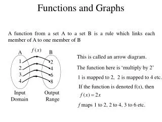
The amount paid is $12 multiplied by the volume of petrol bought 3.1 Introduction to Functions A. Basic Idea of a Function y 12x In this case, we say that y is a function of x. The value of y (the amount paid) depends on a given value of x (the volume of petrol bought). We call y the dependent variable and x the independent variable. Each value of x gives one and exactly one value of y. A variable y is said to be a function of a variable x if there is a relation between x and y such that every value of x gives exactly one value of y.
3.1 Introduction to Functions B. Different Ways to Represent Functions The relation between x and y can be expressed in different ways: Tabular representation Algebraic representation y 12x Graphical representation Plot the corresponding values of x and y according to the above table.
3.1 Introduction to Functions B. Different Ways to Represent Functions Consider a square with side x cm and perimeter y cm. Tabular representation Algebraic representation y 4x Graphical representation Plot the corresponding values of x and y according to the above table. We can use the graph to find the value of y for other value of x, for example: When x 2.5, y 10.
y 3x + 2 and f(x) 3x + 2 represent the same function. Consider the representations f(x) 3x + 2 and y 3x + 2. The meaning of f(10) is the same as that of the phrase ‘the value of y when x 10’. 3.1 Introduction to Functions C. Notation for a Function A function can be expressed by an equation, such as y 3x + 2. It is common to use the notation f(x) to denote a function of x, such as f(x) 3x + 2. Notes: The symbol ‘f(x)’ is read as ‘f of x’, f(x) does not mean f is multiplied by x. f(x) represents the value of the function at x. For example, f(10) is the value of the function f(x) at x 10, that is, f(10) 3(10) + 2 32 The letter ‘f ’ in the notation f(x) may be replaced by other letters to represent different functions of x, such as g(x), h(x), F(x) and G(x).
–19 5 –3 In general, f(a + b) f(a) + f(b). 3.1 Introduction to Functions C. Notation for a Function Example 3.1T Consider f(x) x3 – 4x2 + 5. (a) Find f(–2), f(0) and f(2). (b) Is f(–2) + f(2) f(0)? Solution: (a) f(–2) (–2)3 – 4(–2)2 + 5 (b) f(–2) + f(2) –19 + (–3) –22 and f(0) 5 f(0) (0)3 – 4(0)2 + 5 ∴f(–2) + f(2) f(0) f(2) (2)3 – 4(2)2 + 5
Substitute x 3 into f(x), then find the value of k by solving the equation f(3) 7. k 20 x 2 3.1 Introduction to Functions C. Notation for a Function Example 3.2T Consider f(x) k – 3x2 and f(3) –7. (a) Find the value of k. (b) Find the values of x such that f(x) 8. Solution: (a) f(3) –7 k – 3(3)2 –7 k – 27 –7 (b) From (a), f(x) 20 – 3x2. ∵ f(x) 8 ∴20 – 3x2 8 3x2 12 x2 4
–4a2 – 7a – 2 –4a2+ a + 1 a 3.1 Introduction to Functions C. Notation for a Function Example 3.3T Consider f(x) –4x2 + 7x – 2. (a) Express f(–a) and f(–a + 1) in terms of a. (b) If f(–a) f(–a + 1), find the value of a. Solution: (a) f(x) –4x2 + 7x – 2 f(–a) –4(–a)2 + 7(–a) – 2 f(–a + 1) –4(–a + 1)2 + 7(–a + 1) – 2 –4(a2– 2a + 1) – 7a + 7 – 2 –4a2+ 8a – 4 – 7a + 7 – 2 (b) ∵ f(–a) f(–a + 1) ∴–4a2 – 7a – 2 –4a2+ a + 1 –8a 3
The domain of the function y is the set of all real numbers except 1. Consider g(x) . x cannot be 0. 3.1 Introduction to Functions D. Domain and Co-domain of a Function When describing a function yf(x), we may want to know: (i) Domain all possible values that the independent variable x can take (ii) Co-domain (iii) Range Examples: Consider f(x) x2 + 1. x can take any real numbers. ∴ The domain is the set of all real numbers. ∴ The domain is the set of all real numbers except 0.
For the function yx2 + 1, even though x can be negative, y must be positive. 3.1 Introduction to Functions D. Domain and Co-domain of a Function When describing a function yf(x), we may want to know: (i) Domain all possible values that the independent variable x can take (ii) Co-domain all possible values that the dependent variable y can take (iii) Range all output values of dependent variable y of the function, that is, the corresponding values of independent variable x e.g. Consider f(x) y x2 + 1. (i) Domain: the set of all real numbers (ii) Co-domain: the set of all real numbers (iii) Range: the set of real numbers larger than or equal to 1
Consider g(t) . g(t) is a function of t. 3.1 Introduction to Functions E. Variables in Functions We have been using x and y as the independent and the dependent variables of a function. In fact, we can have functions of other variables: Consider f(l) l2. f(l) is a function of l. Consider h(q) sin q. h(q) is a function of q. We can also use different variables for the same function. For example, f(l) l2, f(x) x2 and f(t) t2 represent the same function. We call the variables l, x and t the dummy variables.
3.2 Quadratic Functions A. Graphs of Quadratic Functions A function in the form yax2 + bx + c, where a, b and c are constants and a 0 is called a quadratic function. Plot the graph of y –x2 – 2x + 6 for –4 x 2: yx2 2x 6 The graph is a curve which is called a parabola.
3.2 Quadratic Functions A. Graphs of Quadratic Functions Example 3.4T Consider yx2 + 2x – 1. (a) Complete the following table. (b) Plotthegraphof yx2+2x–1for –4x2. yx2 2x 1 Solution: (a) yx2 + 2x – 1 (b) Refer to the figure on the right.
3.2 Quadratic Functions B. Properties of Quadratic Functions The following figure shows two parabolas yax2 + bx + c where a > 0 and a < 0 respectively. Each parabola has a vertex. Each parabola is symmetrical about the axis of symmetry. The parabolas cut the y-axis at (0, c) and c is called the y-intercept.
3.2 Quadratic Functions B. Properties of Quadratic Functions Properties of the graph of a quadratic function yax2 + bx + c: 1. Direction of opening: (a) If a > 0, then it opens upwards. (b) If a < 0, then it opens downwards. 2. Since the graph cuts the y-axis at (0, c), c is the y-intercept of the graph. 3. (a) If a > 0, then the vertex is the lowest point of the parabola. (b) If a < 0, then the vertex is the highest point of the parabola. 4. The axis of symmetry passes through the vertex.
3.2 Quadratic Functions B. Properties of Quadratic Functions Apart from determining the direction of opening of the graph, the values of a (in yax2 + bx + c) also affect the width of the opening. When a > 0, the opening is narrower for a larger value of a. When a < 0, the opening is wider for a larger value of a. (i.e., the more negative the value of a, the narrower the opening.)
3.2 Quadratic Functions B. Properties of Quadratic Functions Example 3.5T Consider the graphs of the following three functions: (I) y (x – 3)2 – 1 (II) y 2(x – 3)2 – 1 (III)y –(x – 3)2 + 1 (a) Compare the shapes of the graphs of (I) and (III). (b) Describe thedifferencein theshapesof thegraphsbetween(I)and(II). Solution: (a) Consider function (III): y –(x – 3)2 + 1 –[(x – 3)2 – 1] ∴ (I) and (III) are symmetrical about the x-axis. (b) The coefficients of the x2 terms in (I) and (II) are positive. The coefficient of the x2 term in (II) is greater than that in (I). ∴ The opening of the graph of (I) is wider than that of (II).
3.2 Quadratic Functions C. Solving Quadratic Equations by the Graphical Method Consider the graph of yax2 + bx + c: Suppose the graph cuts the x-axis at two points (p, 0) and (q, 0). The two values p and q are called thex-intercepts of the graph of yax2 + bx + c. Since the y-coordinates of these two points are 0, ax2 + bx + c 0. ∴ The x-intercepts of the graph of yax2 + bx + c satisfy the equation ax2 + bx + c 0. ∴ The x-intercepts of the graph of yax2 + bx + c are the roots of the quadratic equation ax2 + bx + c 0.
3.2 Quadratic Functions C. Solving Quadratic Equations by the Graphical Method Example 3.6T The figure shows the graph of y 5x2 + 8x – 4. Solve 5x2 + 8x – 4 0 graphically. Solution: The graph cuts the x-axis at the points (–2.0, 0) and (0.4, 0). (cor. to the nearest 0.05) Hence the roots of 5x2 + 8x – 4 0 are –2.0 and 0.4.
3.2 Quadratic Functions C. Solving Quadratic Equations by the Graphical Method Example 3.7T The figure shows the graph of y 4x2 + 12x + 9. Solve 4x2 + 12x + 9 0 graphically. Solution: The graph touches the x-axis at the point (–1.5, 0). (cor. to the nearest 0.05) Hence the root of 4x2 + 12x + 9 0 is –1.5.
3.2 Quadratic Functions C. Solving Quadratic Equations by the Graphical Method Example 3.8T The figure shows the graph of y –x2 + x – 1. Solve –x2 + x – 1 0 graphically. Solution: The graph does not intersect with the x-axis. Hence the equation –x2 + x – 1 0 has no real roots.
3.2 Quadratic Functions C. Solving Quadratic Equations by the Graphical Method Example 3.9T Consider the graph of yx2 + 3x + 1. (a) Solve x2 + 3x + 1 0 graphically. (b) Solve the above equation by the quadratic formula and compare the result with (a). Solution: (a) The graph cuts the x-axis at the points (–2.6, 0) and (–0.4, 0). Hence the roots of x2 + 3x + 1 0 are –2.6 and –0.4. (cor. to 1 d. p.) (b) By the quadratic formula, we have According to the scale of the graph, we can only find the approximate roots of the equation correct to 1 decimal place in (a) while the roots in (b) are exact values.
3.2 Quadratic Functions D. Quadratic Graphs and Nature of Roots In Chapter 2, we learnt that the discriminant D of a quadratic equation can help us to determine the nature of the roots. We can also use Db2 – 4ac to find the number of x-intercepts of the graph of yax2 + bx + c. If Db2 – 4ac > 0, then the graph of yax2 + bx + ccuts the x-axis at two distinct points. If Db2 – 4ac 0, then the graph of yax2 + bx + ctouches the x-axis at only one point. If Db2 – 4ac < 0, then the graph of yax2 + bx + c does not cut the x-axis.
3.2 Quadratic Functions D. Quadratic Graphs and Nature of Roots The following table summarizes the nature of roots of quadratic equations and the corresponding number of x-intercepts of their graphs.
k 6 x –2 3.2 Quadratic Functions D. Quadratic Graphs and Nature of Roots Example 3.10T The graph of y (2 – k)x2 – 16x – 16 touches the x-axis at only one point. (a) Find the value of k. (b) Hence solve (2 – k)x2 – 16x – 16 0. Solution: (a) Since the graph touches the x-axis, D 0. 162 – 4(2 – k)(–16) 0 256 + 128 – 64k 0 64k 384 (b) The equation is –4x2 – 16x – 16 0. ∴x2+ 4x+ 4 0 (x+ 2)2 0
m 0 m 0 3.3 Graphs of Other Functions A. Linear Functions A function in the form ymx + c, where m and c are constants and m 0 is called a linear function. Notes: c is the y-intercept of the graph. If c 0, then the graph is a straight line passing through the origin. If m 0, then the function becomes y c which is called a constant function.
3.3 Graphs of Other Functions B. Other Functions Apart from linear and quadratic functions, Example 3.11T and Example 3.12T show some other functions.
The function yax3 + bx2 + cx + d, where a, b, c and d are constants and a 0, is called a cubic function. 3.3 Graphs of Other Functions B. Other Functions Example 3.11T Consider the function yx3 – 2x2 – x + 2. (a) Plot the graph of yx3 – 2x2 – x + 2 for –2 x 3. (b) Find the x-intercepts and the y-intercept of the graph. (Give the answers correct to 1 decimal place if necessary.) Solution: (a) (b) The x-intercepts are–1.0, 1.0 and 2.0. The y-intercept is 2.0.
The figure shows the graphs of y 3(2 – x), yx2 + 9 and y – 2. Compare the graphs of the functions with respect to the following: (a) domain (b) existence of maximum or minimum value (c) number of x-intercepts For y – 2, the domain is the set of all real numbers except 0. 3.3 Graphs of Other Functions B. Other Functions Example 3.12T Solution: (a) For y 3(2 – x), the domain is the set of all real numbers. For yx2 + 9, the domain is the set of all real numbers.
The figure shows the graphs of y 3(2 – x), yx2 + 9 and y – 2. Compare the graphs of the functions with respect to the following: (a) domain (b) existence of maximum or minimum value (c) number of x-intercepts For y – 2, there is no maximum or minimum value. For y – 2, there is one x-intercept. 3.3 Graphs of Other Functions B. Other Functions Example 3.12T Solution: (b) For y 3(2 – x), there is no maximum or minimum value. For yx2 + 9, there is a minimum value. (c) For y 3(2 – x), there is one x-intercept. For yx2 + 9, there is no x-intercept.
Chapter Summary 3.1 Introduction to Functions 1. A variable y is said to be a function of x if there is a relation between x and y such that every value of x corresponds to exactly one value of y. 2. We use f(x) to denote a function of x, where x is the independent variable. 3. The domain is the set of values that the independent variable can take. The co-domain is the set of possible values that the dependent variable can take. The range is the set of values that the dependent variable takes corresponds to the independent variable.
Chapter Summary 3.2 Quadratic Functions Properties of the graph of yax2 + bx + c: 1. (a) If a > 0, then the graph opens upwards. (b) If a < 0, then the graph opens downwards. 2. The graph cuts the y-axis at (0, c), that is, the y-intercept c. 3. The vertex is the turning point of the graph. (a) If a > 0, the vertex is the minimum point of the graph. (b) If a < 0, the vertex is the maximum point of the graph. 4. The axis of symmetry is a line that the graph is symmetrical about it. It passes through the vertex of the graph.
Chapter Summary 3.2 Quadratic Functions For two quadratic functions: (I) ya1x2 + b1x + c1 (II) ya2x2 + b2x + c2 If 0 < a1 < a2 or 0 > a1 > a2, then graph (II) opens narrower than the graph (I). The roots of the quadratic equation ax2 + bx + c 0 (a 0) can be obtained by finding the x-intercept(s) of the graph.
Chapter Summary 3.3 Graphs of Other Functions 1. The graph of a linear function ymx + cis a straight line. 2. Without drawing the graph of a function yf(x), they-intercept can be found by putting x 0 into the function, that is, the y-intercept of yf(x) is f(0).
