Density Functional Theory
Density Functional Theory. 15.11.2006. 1920. 1940. 1960. 1980. 2000. 2020. 1900. A long way in 80 years. L. de Broglie – Nature 112, 540 (1923). E. Schrodinger – 1925, …. Pauli exclusion Principle - 1925. Fermi statistics - 1926. Thomas-Fermi approximation – 1927


Density Functional Theory
E N D
Presentation Transcript
Density Functional Theory 15.11.2006
1920 1940 1960 1980 2000 2020 1900 A long way in 80 years • L. de Broglie – Nature 112, 540 (1923). • E. Schrodinger – 1925, …. • Pauli exclusion Principle - 1925 • Fermi statistics - 1926 • Thomas-Fermi approximation – 1927 • First density functional – Dirac – 1928 • Dirac equation – relativistic quantum mechanics - 1928
1920 1940 1960 1980 2000 2020 1900 Quantum Mechanics TechnologyGreatest Revolution of the 20th Century • Blochtheorem – 1928 • Wilson - Implications of band theory - Insulators/metals –1931 • Wigner- Seitz – Quantitative calculation for Na - 1935 • Slater - Bands of Na - 1934 (proposal of APW in 1937) • Bardeen - Fermi surface of a metal - 1935 • First understanding of semiconductors – 1930’s • Invention of the Transistor – 1940’s • Bardeen – student of Wigner • Shockley – student of Slater
1920 1940 1960 1980 2000 2020 1900 The Basic Methods of Electronic Structure • Hylleras – Numerically exact solution for H2 – 1929 • Numerical methods used today in modern efficient methods • Slater – Augmented Plane Waves (APW) - 1937 • Not used in practice until 1950’s, 1960’s – electronic computers • Herring – Orthogonalized Plane Waves (OPW) – 1940 • First realistic bands of a semiconductor – Ge – Herrman, Callaway (1953) • Koringa, Kohn, Rostocker – Multiple Scattering (KKR) – 1950’s • The “most elegant” method - Ziman • Boys – Gaussian basis functions – 1950’s • Widely used, especially in chemistry • Phillips, Kleinman, Antoncik,– Pseudopotentials – 1950’s • Hellman, Fermi (1930’s) – Hamann, Vanderbilt, … – 1980’s • Andersen – Linearized Muffin Tin Orbitals (LMTO) – 1975 • The full potential “L” methods – LAPW, ….
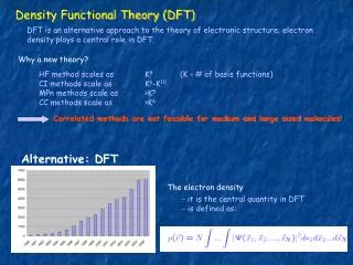
1920 1940 1960 1980 2000 2020 1900 Basis of Most Modern CalculationsDensity Functional Theory • Hohenberg-Kohn; Kohn-Sham - 1965 • Car-Parrinello Method – 1985 • Improved approximations for the density functionals • Evolution of computer power • Nobel Prize for Chemistry, 1998, Walter Kohn • Widely-used codes – • ABINIT, VASP, CASTEP, ESPRESSO, CPMD, FHI98md, SIESTA, CRYSTAL, FPLO, WEIN2k, . . .
electrons in an external potential Interacting
The basis of most modern calculationsDensity Functional Theory (DFT) • Hohenberg-Kohn (1964) • All properties of the many-body system are determined by the ground state density n0(r) • Each property is a functional of the ground state density n0(r) which is written as f [n0] • A functional f [n0] maps a function to a result: n0(r) →f
The Kohn-Sham Ansatz • Kohn-Sham (1965) – Replace original many-body problem with an independent electron problem – that can be solved! • The ground state density is required to be the same as the exact density • Only the ground state density and energy are required to be the same as in the original many-body system
Exchange-CorrelationFunctional – Exact theorybut unknown functional! Equations for independentparticles - soluble The Kohn-Sham Ansatz II • From Hohenberg-Kohn the ground state energy is a functional of the density E0[n], minimum at n = n0 • From Kohn-Sham • The new paradigm – find useful,approximate functionals
Numerical solution: plane waves • Kohn-Sham equations are differential equations that have to be solved numerically • To be tractable in a computer, the problem needs to be discretized via the introduction of a suitable representation of all the quantities involved • Various discretization approeches. Most common are Plane Waves (PW) and real space grids. • In periodic solids, plane waves of the form are most appropriate since they reflect the periodicity of the crystal and periodic functions can be expanded in the complete set of Fourier components through orthonormal PWs • In Fourier space, the K-S equations become • We need to compute the matrix elements of the effective Hamiltonian between plane waves
Numerical solution: plane waves • Kinetic energy becomes simply a sum over q • The effective potential is periodic and can be expressed as a sum of Fourier components in terms of reciprocal lattice vectors • Thus, the matrix elements of the potential are non-zero only if q and q’ differ by a reciprocal lattice vector, or alternatively, q = k+Gm and q’ = k+Gm’ • The Kohn-Sham equations can be then written as matrix equations • where: • We have effectively transformed a differential problem into one that we can solve using linear algebra algorithms!
Input parameters: &electrons • Kohn-Sham equations are always self-consistent equations: the effective K-S potential depends on the electron density that is the solution of the K-S equations • In reciprocal space the procedure becomes: • Iterative solution of self-consistent equations - often is a slow process if particular tricks are not used: mixing schemes where and