Density Functional Theory: a first look
Density Functional Theory: a first look . Patrick Briddon. Theory of Condensed Matter Department of Physics, University of Newcastle, UK. Contents. Density Functional Theory Hohenberg Kohn Theorems Thomas Fermi Theory Kohn-Sham Equations Self Consistency Approximations for E xc .


Density Functional Theory: a first look
E N D
Presentation Transcript
Density Functional Theory: a first look Patrick Briddon Theory of Condensed Matter Department of Physics, University of Newcastle, UK.
Contents Density Functional Theory • Hohenberg Kohn Theorems • Thomas Fermi Theory • Kohn-Sham Equations • Self Consistency • Approximations for Exc.
Density Functional Theory Work with n(r) instead of Standard approach of QM : DFT : work in terms of density : N.B. : few IFs and BUTs here
3 Important Questions Three important questions: • Can we really write E[n]? • If so, how can we find n(r)? • What is the functional E[n] ?
1st Hohenberg Kohn Theorem The external potential V(r) is determined to within a constant by the ground state charge density of a system. i.e. one-to-one relationship This is an astonishing statement! Why?
1st Hohenberg Kohn Theorem Proof: Suppose we have two systems Hamiltonians H1, H2 External potentials V1 , V2 GS wavefunctions: Y1, Y2 But the same GS density n(r)
We clearly have But: So: Swap 1 and 2: Contradiction!
Our starting point was wrong! We cannot have two different systems with the same GS density. Importance of this: we can write E[n]. Now move on the second question – how can we find the density? Hohenberg – Kohn’s second theorem.
2nd Hohenberg Kohn Theorem “The true ground state charge density is that which minimises the total energy.” An equivalent to the usual variational principle of quantum mechanics.
Proof We have (variational principle) Define Then
Some problems V-representability (only minimise over densities which can arise from GS wavefunctions of real systems Levy showed that the densities need only satisfy a weaker condition that they can be obtained from an antisymmetric wavefunction (N-representable). n must be +ve, continuous, normalised
Some extensions Spin dependent potentials e.g. magnetic fields E[n] E[n, n - n] or E[n, n] Main advantage: better description of open shell systems.
3 Important Questions Three important questions: • Can we really write E[n]? • If so, how can we find n(r)? • What is the functional E[n] ? Now for the last question. What is the formula!
What is the functional? Difficult : still not answered exactly! Problem is that other two terms are very large - any attempt at approximation must be good.
Thomas-Fermi Method Classical expression for electron- electron term:
Thomas-Fermi Method Statistical idea for KE based on uniform electron gas result: KE per electron =
Thomas-Fermi Method What about a non uniform system? A. Assume that things vary slowly: DV r Total is thus
Thomas-Fermi Method Final energy is thus: How useful is this?
Thomas-Fermi Method • What is the conclusion? • Energies quite good (error < 1%). • Difference of energies not good enough to describe bonding. • How can we improve this?
Thomas-Fermi Method • Add exchange/correlation (missing do far). • Try to take account of non-uniform system. • Write T[n] as T[n, grad |n|] • All failures!
Kohn-Sham methodPhys Rev 140, 1133A (1966) Realised that approximation must be made to terms that are small: KE is big! Improving T[n] did not work. Need a completely different approach. Second half of HK paper therefore discarded.
Kohn-Sham methodPhys Rev 140, 1133A (1966) Introduce a system which: 1. Is non-interacting 2. Has same n(r) as the real system. [non-interacting N-representability - an assumption! ]
Kohn-Sham contd. where Ts[n] is the KE of the non-interacting system and the final term, T, is small.
Kohn-Sham contd. • Exc[n] includes both T and contributions to el-el energy beyond the Hartree term. • The key hope is that this is • small • less sensitive to external potential • These mean differences are accurate.
We now have two questions: (a) how to find Ts[n] ? (b) what is Exc[n] ? For a non-interacting system it is exactly true that the many electron wavefunction is a single Slater determinant.
For this: and:
The (r) must be found from a self consistent solution of: These are called the Kohn-Sham equations. Solve iteratively:
Guess: Construct Solve Find new density: Look at Form a better input and continue.
Self Consistent Cycle • This process is called the self-consistent cycle. • Starting guess is a superposition of atomic charge densities (or a restart dump). • AIMPRO produces output showing how the energy converged and how the input and output densities come together.
AIMPRO SCF etot,echerr 1 -1.1289007706 0.0547166884 0.884981 2.95 106.1 120.7 etot,echerr 2 -1.1319461182 0.0303263020 0.488911 3.05 106.1 120.7 etot,echerr 3 -1.1361047998 0.0000338275 0.000689 3.00 106.1 120.7 etot,echerr 4 -1.1360826939 0.0001723143 0.002700 2.99 106.1 120.7 etot,echerr 5 -1.1361076063 0.0000002649 0.000004 3.00 106.1 120.7 • The numbers are: • Total energy (reduces to converged value) • 2 measures of • Time taken per iteration • Current memory being used (MB) • Max memory used so far (MB)
Kohn-Sham Levels We got the Kohn Sham eqn: Q: what exactly are the el and jl? A: the eigenvalues and eigenfunctions of a ficticious non-interacting system which has the same density as the real system.
KS Levels Contd. They are not the energies of quasiparticles. Typical semiconductor results: Lattice constant to 1% Bulk modulus to 1% Phonon frequencies to 5% LDA “gap” for Si is 0.6eV; 0.1 eV for Ge!
KS Levels Contd. Bandstructures are qualitatively correct. (Scissors operator). Physical nature of the KS eigenfunctions sensible. P in Si - get state just below conduction band Dangling bonds - localised states in mid gap.
AIMPRO and KS levels spin, kpoint : 1 1 1 -10.0938 1.2658 3.7422 3.7422 5.9056 8.7912 2.0000 0.0000 0.0000 0.0000 0.0000 0.0000 The KS levels in eV. Used in “bandstructure” plots. Occupancies also given (this is a spin averaged calculation)
3 Important Questions Three important questions: • Can we really write E[n]? • If so, how can we find n(r)? • What is the functional E[n] ? • All remaining questions are in Exc[n]. Now finally we look at what this is.
Exchange correlation energy Our DFT total energy is: What about the last term?
The Local Density Approximation (LDA) Write where exc(n) is the exchange-correlation energy per electron for a uniform electron gas. This seems a bit rough and very similar to Thomas Fermi, but this term is now very much smaller.
Exc for Homogeneous electron gas • By simple analytical treatment for the exchange energy. • Using many body perturbation theory (for various limits of correlation energy) • By looking at quantum Monte-Carlo calculations and parametrising them • Intelligent interpolation between these
Exc for Homogeneous electron gas contd. Simple analysis for exchange part gives • Correlation is harder, see:: • Perdew Zunger (1981) • Vosko, Wilk, Nusair (1980) • Perdew, Wang (1992)
Simple Tests : Molecules Example : water H20
Simple tests : solids • Standard “bulk” calculations : • lattice constant (Si : 1%) • bulk modulus (Si : 2%) • phonon spectra (2 %) • formation energies (LDA : 20 %) • excitation energies (50 %)
Phonon Spectrum Material : GaAs. All frequencies in cm-1
How to Improve? Next step is to move beyond the LDA: The Gradient expansion Approximation (GEA). Early history of these was bad. Calculations made worse, not better.
Generalised Gradient Approximations (GGA) • Sum rules are obeyed correctly • scaling behaviour of exchange correlation energy correct • Various limiting forms • Bounds (Lieb-Oxford) Idea is to ensure that
Popular GGAs • B88 (empirical, chemistry) • BLYP (chemistry) • PW91 (physics, poor form) • PBE96 (physics, easier to use)
Generalised Gradient Approximations (GGA) • In general, GGA weakens bonds slightly. • It improves results for: • binding energies of molecules • description of surfaces • H-bonding
THE CONCLUSION • An absolutely huge success • 1988 two groups in UK doing DFT • Cambridge (TCM) • Exeter • Today: every department? • Chemistry/engineering too! • Applications in huge variety of areas.
Work to do! • Kittel Ch 6: “Free Electron Fermi Gas” • Hohenberg and Kohn, PR (1964) • Kohn-Sham, PR (1965) • Perdew Zunger, PRB (1981) • Perdew, Wang, PRB (1992) • Perdew, Burke, Enzerhoff PRL (1996)